Teaching an LLM to Explore: Reinforcement Learning for Document Navigation
Authors: Mohammed Alshehri
Year: 2026
TL;DR: We trained a Qwen3-8B model to efficiently search through documents using GRPO, inspired by Karpathy's autoresearch — and what Goodhart's Law taught us along the way.
- Lower training reward = better model: the run with the lowest training reward produced the best model.
- Goodhart's Law in action: shaped rewards created a shortcut the agent exploited while ignoring the true objective.
- Status text fix was the breakthrough: 50% of outputs were action descriptions instead of answers.
- Tinker-Explorer: an RL environment for multi-hop document exploration with budget-constrained action space.
- Three-run ablation demonstrating that reward quality matters more than reward quantity in GRPO training.
- Practical diagnosis of status-text pollution as a dominant failure mode invisible in aggregate metrics.
- Evidence that sparse but honest reward signals outperform dense but misleading ones.
We present Tinker-Explorer, a reinforcement learning agent that learns to navigate document chunks to answer multi-hop questions, trained using GRPO on the Tinker platform. Inspired by Karpathy's autoresearch, the agent operates under a step budget, deciding which documents to read before answering. Across three training runs, we demonstrate a Goodhart's Law failure (shaped rewards degrading performance), diagnose a status-text pollution problem invisible in aggregate metrics, and show that the run with the lowest training reward produced the best model (F1 = 0.172, 40% improvement over Run 1). The central insight: reward quality matters more than reward quantity.
Teaching an LLM to Explore: Reinforcement Learning for Document Navigation
How we trained a Qwen3-8B model to efficiently search through documents using GRPO, inspired by Karpathy’s autoresearch — and what Goodhart’s Law taught us along the way.
Table of Contents
- Introduction — The Autoresearch Connection
- The Problem: Partially Observable Multi-Hop QA
- Environment Design
- The Dataset: 2WikiMultiHopQA
- Training Infrastructure: Tinker + GRPO
- Run 1: Shaped Reward — The Goodhart Trap
- Run 2: Pure F1 — Cleaning the Signal
- Run 3: Status Text Fix — The Breakthrough
- The Paradox: Lower Training Reward = Better Model
- Results and Analysis
- Lessons Learned
- What's Next
1. Introduction — The Autoresearch Connection
In March 2025, Andrej Karpathy announced autoresearch — a project where an AI agent autonomously improves a language model by searching over code edits, running experiments within a 5-minute budget, and optimizing validation perplexity. The core insight was simple but profound: give an agent a search space, a budget, and a scalar reward, then let reinforcement learning do the rest.
Karpathy’s search space was code modifications. Ours is something different: document exploration.
We built Tinker-Explorer, an RL agent that learns to navigate a set of document chunks to answer multi-hop questions. Like autoresearch, it operates under a budget (limited steps), must decide what information to gather (which documents to read), and receives a scalar reward (answer correctness). Unlike autoresearch, the search space isn’t code — it’s evidence.
The mapping between the two projects:
| Karpathy's Autoresearch | Tinker-Explorer | |
|---|---|---|
| Agent | Code-editing LLM | Document-exploring LLM |
| Search space | Code modifications | Document chunk selections |
| Budget | 5 minutes wall-clock | 10 action steps max |
| Reward | val_bpb improvement | Token F1 on answer |
| Optimization | RL over code edits | GRPO over exploration trajectories |
| Key challenge | Which edits improve the model? | Which documents contain the answer? |
Both projects share the same fundamental question: Can an LLM learn to make better decisions about what to explore, through trial and error?
This post documents our journey across three training runs — including a Goodhart’s Law failure, a reward debugging mystery, and the realization that looking at your model’s actual outputs matters more than tuning hyperparameters.
2. The Problem: Partially Observable Multi-Hop QA
Standard QA gives the model everything upfront. Retrieval-augmented QA retrieves documents first, then answers. But neither captures the active information gathering that humans do naturally.
Consider this question:
“Which film has the director born first, Once A Gentleman or The Girl In White?”
A human researcher would: look at the available sources, open the article about “Once A Gentleman” to find the director’s birth year, open the article about “The Girl In White” to do the same, then compare the two dates and answer.
This process requires sequential decision-making under uncertainty — the agent doesn’t know which documents are useful until it reads them. This is fundamentally a reinforcement learning problem.
Why Not Just Retrieve Everything?
You could argue: “Just open all the documents.” But in real-world settings, API calls cost money (think: calling a paid knowledge base), context windows have limits, irrelevant information introduces noise that degrades LLM performance, and some documents are red herrings that actively mislead.
The goal isn’t just to answer correctly — it’s to answer correctly while reading as few documents as possible. This is the efficiency-accuracy tradeoff that makes the problem interesting.
3. Environment Design
Tinker-Explorer implements a standard RL environment loop:
State Space
At each step, the agent observes:
The question (e.g., “Who is Marie Zéphyrine Of France’s paternal grandmother?”)
A list of chunk previews — one-line titles of all available documents, but NOT their contents
Previously opened chunks — full text of any documents the agent has chosen to read
Remaining step budget — how many actions it has left
Action Space
Three possible actions at each step:
{"action": "OPEN", "target": 3, "reasoning": "Chunk 3 mentions Marie Zéphyrine..."}
{"action": "SUMMARIZE", "target": 3, "text": "Born 1750, daughter of Louis XV..."}
{"action": "ANSWER", "text": "Marie Leszczyńska"}
OPEN(i) — Read chunk i’s full text. This is the exploration action.
SUMMARIZE(i) — Write a summary of chunk i. This helps manage context length.
ANSWER(text) — Submit a final answer. Ends the episode.
Reward Function
The agent receives reward only when it answers. The reward is the token-level F1 score between its predicted answer and the gold answer — a standard metric from the SQuAD literature that gives partial credit for overlapping words.
For example:
Gold: “The Mask Of Fu Manchu” → Predicted: “The Mask of Fu Manchu” → F1 = 1.0 ✅
Gold: “Małgorzata Braunek” → Predicted: “Chunk 4 has been opened” → F1 = 0.0 ❌
Episode Flow
1. Agent receives question + chunk previews
2. Agent decides: OPEN, SUMMARIZE, or ANSWER?
3. If OPEN/SUMMARIZE → environment reveals text, step counter increments
4. If ANSWER → episode ends, reward = token_f1(predicted, gold)
5. If step budget exhausted → episode ends with reward = 0
A typical successful episode takes 2-4 steps: open the relevant chunks, then answer.
4. The Dataset: 2WikiMultiHopQA
We use 2WikiMultiHopQA — a multi-hop question answering dataset built from Wikipedia. Each question requires reasoning across exactly two Wikipedia articles.
Why this dataset?
Natural chunk structure — Each Wikipedia article is a chunk. The agent must decide which articles to read.
Ground truth supporting facts — The dataset provides supporting_facts — which paragraphs contain the answer evidence. This lets us measure whether the agent opens the right documents.
Multi-hop reasoning — Questions require combining information from two sources. The agent can’t answer from a single document.
Varied question types — Comparison (“which film came first”), bridge (“who is the mother of the director of…”), and compositional questions.
Dataset Split
Training: 5,000 tasks (randomly sampled from the full 167K)
Validation: 200 held-out tasks for evaluation
Chunk pool: Each task has ~10 candidate chunks (2 relevant, ~8 distractors)
5. Training Infrastructure: Tinker + GRPO
Tinker Platform
All training runs on Tinker (Temporal Intelligence via Neural Knowledge Extraction and Reasoning) — a cloud platform that provides:
Hosted model weights — Qwen3-8B with LoRA adapters, no local GPU needed
Sampling API — generate completions from the current policy
Training API — submit gradient updates (importance-sampled policy gradient)
Checkpointing — save/restore model states
This architecture is powerful: the model lives in the cloud, and our local code just orchestrates rollouts and computes gradients. We ran all experiments on a MacBook with no GPU.
GRPO (Group Relative Policy Optimization)
We use GRPO — a variant of policy optimization from DeepSeek-R1 — instead of PPO. The key idea:
For each task, sample G = 16 trajectories from the current policy. Compute rewards for all 16. Normalize rewards within the group: advantage_i = (r_i - mean(r)) / std(r). Update the policy to increase probability of above-average trajectories.
Why GRPO over PPO?
No value function needed — PPO requires a separate critic network. GRPO computes baselines from the group.
Natural for language — each trajectory is a sequence of tokens. GRPO treats the whole sequence as one “action.”
Simpler implementation — just a weighted policy gradient update, no GAE, no clipping ratio (handled by importance sampling).
Hyperparameters
| Parameter | Value | Rationale |
|---|---|---|
| GROUP_SIZE | 16 | Balance between variance reduction and compute |
| BATCH_SIZE | 8 | Tasks per batch (= 128 total rollouts per update) |
| Learning Rate | 5e-6 | Conservative — RL fine-tuning is sensitive |
| LoRA Rank | 32 | Enough capacity without overparameterizing |
| Grad Clip Norm | 1.0 | Prevents IS loss explosions |
| Max Steps | 10 | Episode timeout |
SFT Warm-Start
Before RL training, we performed supervised fine-tuning (SFT) on 450 demonstration episodes generated by a heuristic policy. This gives the model a reasonable starting point — it knows the action format and basic exploration strategy.
The heuristic policy simply: computes TF-IDF overlap between the question and each chunk title, opens the highest-overlap chunk, and answers with the chunk title (which is often the Wikipedia article title — and therefore the exact entity name).
This heuristic achieves F1 = 0.246 — a surprisingly strong baseline.
6. Run 1: Shaped Reward — The Goodhart Trap
Hypothesis
“If we add a bonus for opening relevant chunks, the model will learn to explore more effectively.”
Reward Design
reward = token_f1(predicted, gold) + 0.2 × (number of relevant chunks opened)The idea was sound: reward the agent not just for the final answer, but for the intermediate exploration steps. Every relevant chunk opened earns a +0.2 bonus (capped at 0.4).
Training
100 batches over ~12 hours. Training reward climbed steadily — the 5-batch average increased from 0.08 to 0.20 over the course of training.
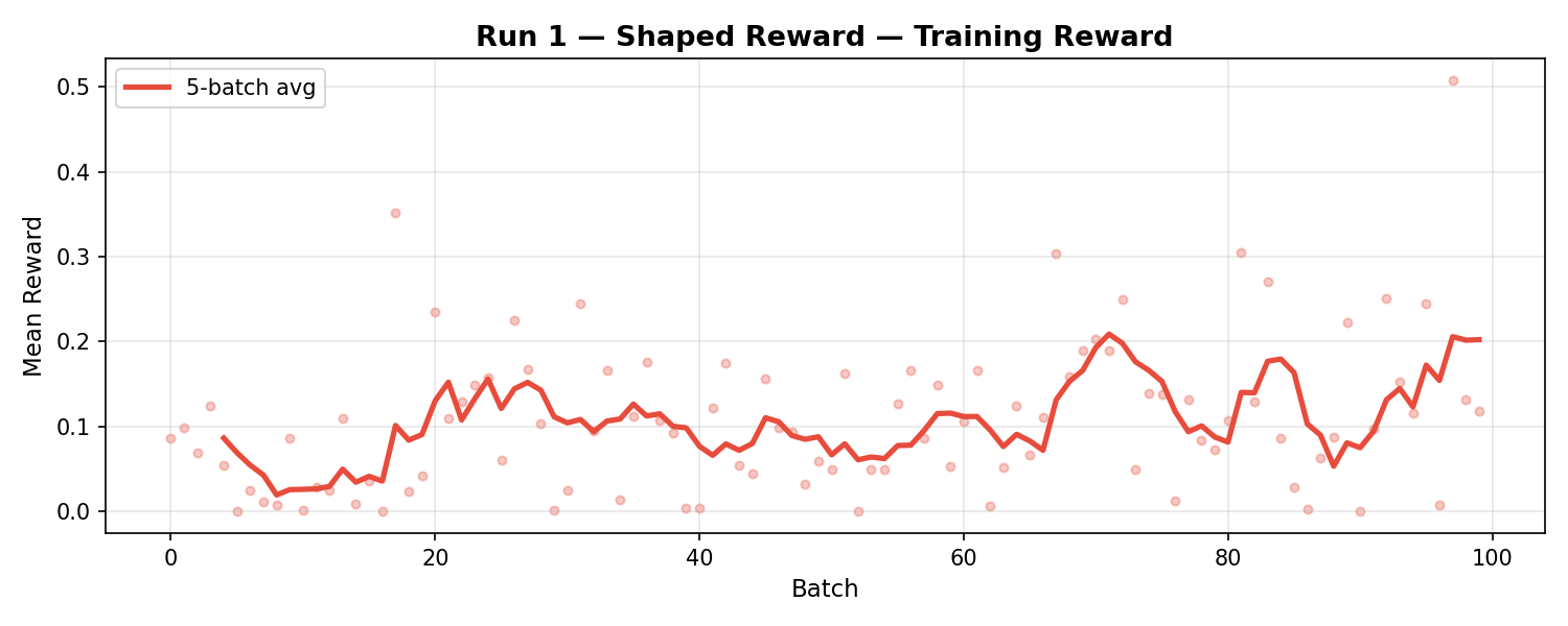
Run 1 Training Reward</figcaption> </figure>
Results
| Model | F1 | EM | Answer Rate |
|---|---|---|---|
| Heuristic | 0.246 | 0.220 | 100% |
| SFT | 0.152 | 0.065 | 87% |
| RL Run 1 | 0.123 | 0.010 | 96% |
Wait — F1 went DOWN? The RL agent performed worse than the SFT baseline it started from. Training reward increased, but actual answer quality decreased.
The Diagnosis: Goodhart’s Law
“When a measure becomes a target, it ceases to be a good measure.”
The relevance bonus created a shortcut: the agent learned to open the right chunks (earning the +0.2 bonus) while paying less attention to actually answering correctly. The training reward was dominated by the exploration bonus, not answer quality — so the gradient signal pushed the model to optimize opens, not answers.
This is a textbook case of reward hacking. The agent found a way to earn high reward without doing the thing we actually wanted (accurate answers).
Goodhart’s Law Visualization — the inverse relationship between training reward and model quality</figcaption> </figure>
Lesson
Shaped rewards are dangerous. The extra signal might seem helpful, but if it’s easier to optimize than the true objective, the agent will chase the bonus and ignore what matters.
7. Run 2: Pure F1 — Cleaning the Signal
The Fix
Strip everything back to the minimum:
reward = token_f1(predicted, gold) # nothing elsePlus one safety gate: the agent must open at least 1 chunk before earning any reward. This prevents the degenerate strategy of answering immediately without reading anything.
Training
100 batches. Immediately obvious: training reward was lower than Run 1. The agent earned less reward per batch because there was no easy bonus to collect.
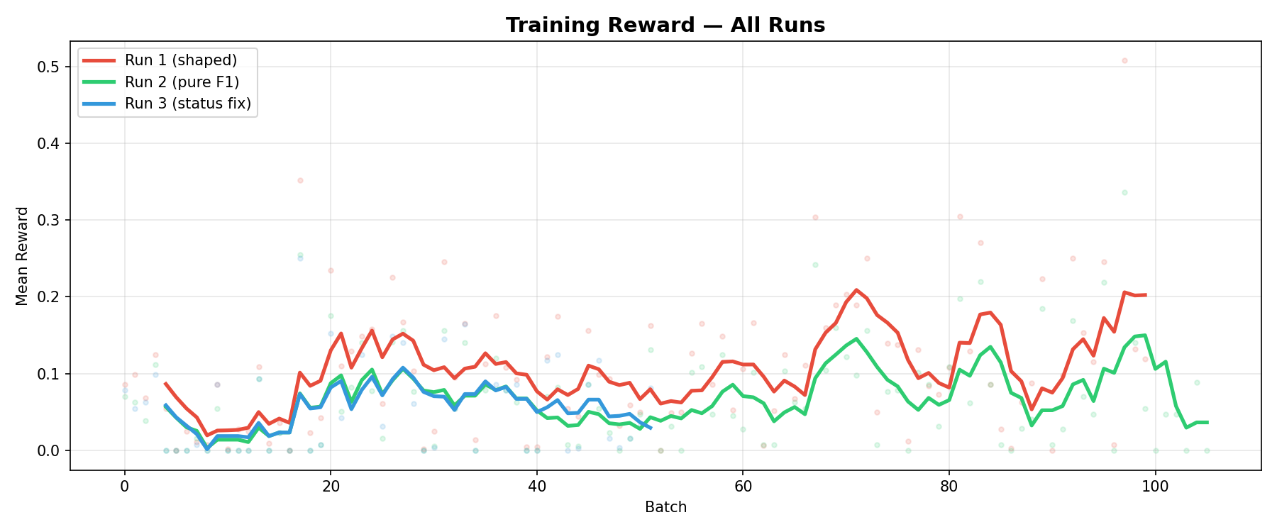
All training reward curves across three runs — lower training reward correlated with better model quality</figcaption> </figure>
The red line (Run 1) sits higher than the green line (Run 2) throughout training. To someone only watching the training curves, Run 1 looks better. But…
Results
| Model | F1 | EM | Answer Rate |
|---|---|---|---|
| Heuristic | 0.246 | 0.220 | 100% |
| SFT | 0.152 | 0.065 | 87% |
| RL Run 1 (shaped) | 0.123 | 0.010 | 96% |
| RL Run 2 (pure F1) | 0.154 | 0.065 | 89.5% |
F1 jumped from 0.123 to 0.154 — a 25% improvement — by removing reward signal. The pure F1 agent matched the SFT baseline, which means the RL training at least didn’t hurt, even if it didn’t help much.
Error Analysis
We looked at what the model actually output on the 200 val tasks:
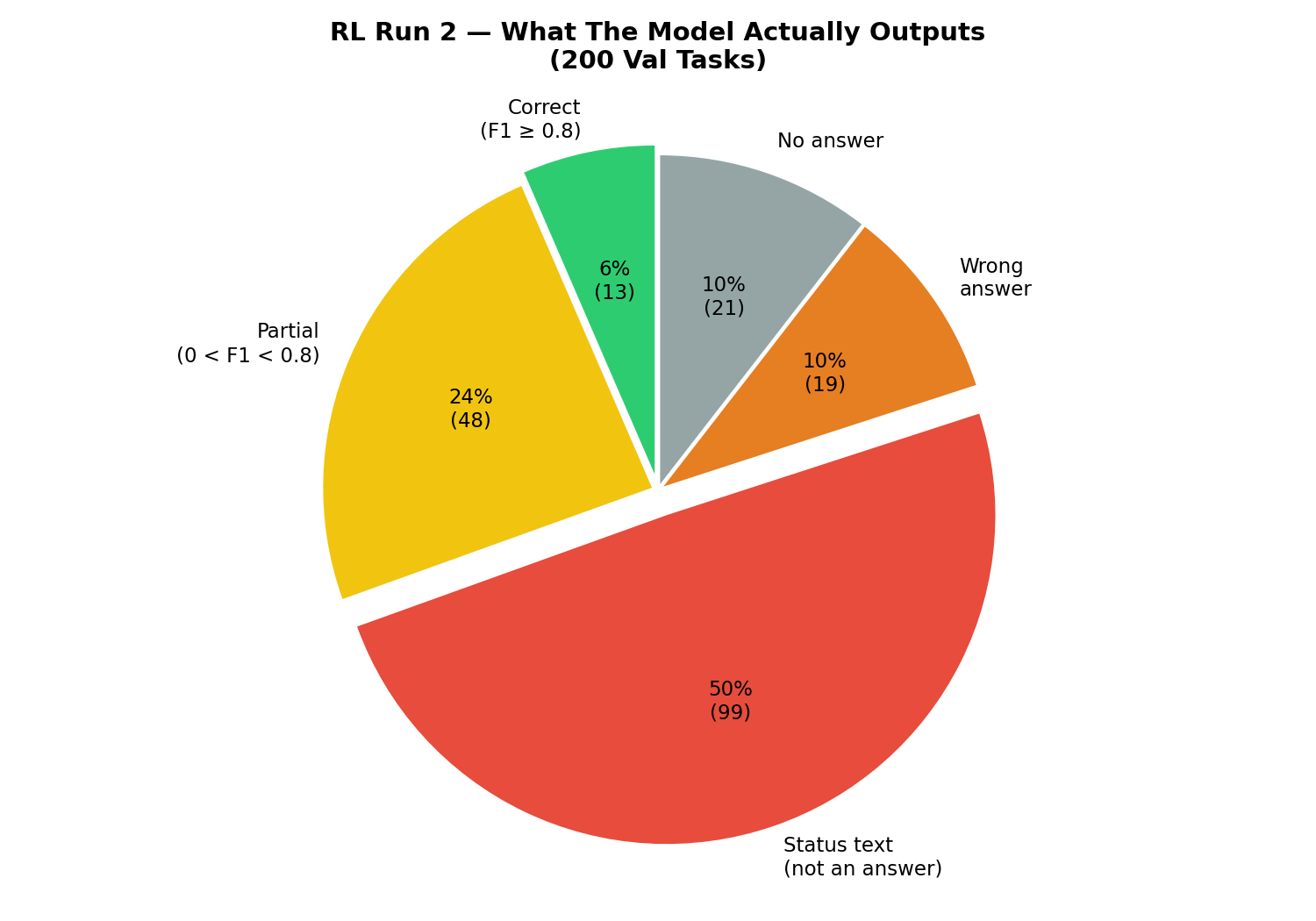
Prediction breakdown showing 50% of outputs were status text instead of answers</figcaption> </figure>
50% of outputs were status text — things like: “Chunk(s) 4 and 7 (‘Polish-Russian War’ and ‘Xawery Żuławski’) have been opened.” or “Chunk 0 (‘Blind Shaft’) has highest overlap with the question.”
The model was outputting descriptions of its own actions instead of answers. It opened the right chunks, formed the right reasoning — then put the reasoning in the answer field instead of the actual answer.
This error mode is invisible in aggregate metrics. You can only find it by reading examples.
8. Run 3: Status Text Fix — The Breakthrough
The Insight
The 50% status text rate meant that half our training signal was wasted. These episodes generated zero reward (because “Chunk 4 has been opened” has zero token overlap with “Małgorzata Braunek”) — but the model didn’t learn from them because the gradient signal was the same as for genuinely wrong answers.
We needed to make the punishment explicit.
Three Changes
1. Reward penalty — If the answer starts with known status text patterns, force reward to 0:
_STATUS_PREFIXES = ("chunk", "the chunk", "chunks", "i have", "i've", "based on")

if any(answer_text.lower().startswith(p) for p in _STATUS_PREFIXES):
    return 0.0  # you gave me reasoning, not an answer
2. Prompt update — Added an explicit “NEVER do this” section:
NEVER put any of these in the "text" field:
- "Chunk X has been opened" — this is NOT an answer
- "Chunk X has highest overlap" — this is reasoning, not an answer
- "Based on the text..." — just give the answer directly
3. Same pure F1 base — No relevance bonus. Min-read gate still active.
Training
~102 batches across two sessions (the first session crashed at batch 52 due to a Tinker API network timeout; we resumed from the batch 50 checkpoint).
Training reward was the lowest of all three runs — the status text penalty made the signal even sparser (71% nonzero batches, vs 78% in Run 2 and 96% in Run 1).
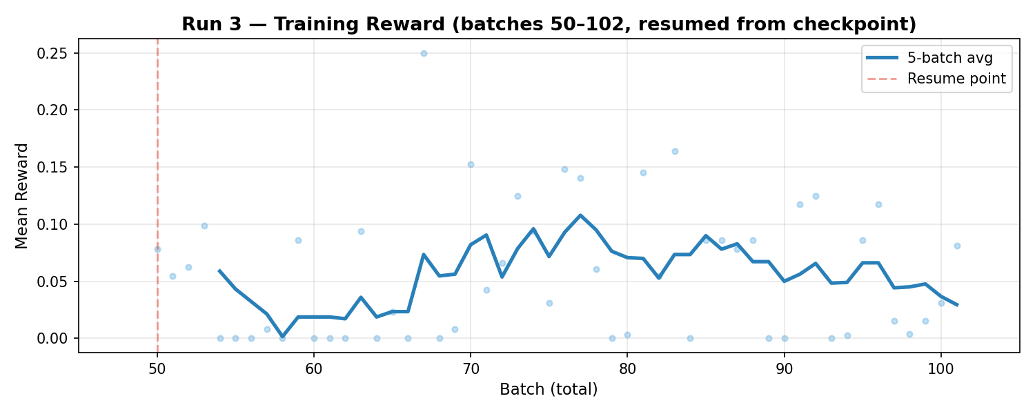
Run 3 Training Reward — lowest training reward, but best model</figcaption> </figure>
Results
| Model | F1 | EM | Answer Rate | Avg Opens |
|---|---|---|---|---|
| Heuristic | 0.246 | 0.220 | 100% | 1.2 |
| SFT | 0.142 | 0.060 | 87.0% | 1.6 |
| RL Run 1 (shaped) | 0.123 | 0.010 | 96.0% | 1.4 |
| RL Run 2 (pure F1) | 0.154 | 0.065 | 89.5% | 1.5 |
| RL Run 3 (status fix) | 0.172 | 0.085 | 99.5% | 1.2 |
🎉 Best results across every metric:
F1 = 0.172 — 40% better than Run 1, 21% better than SFT
EM = 0.085 — 8.5× better than Run 1
Answer Rate = 99.5% — the model almost always gives an answer now
Efficiency = 1.2 opens — same as the heuristic, better than SFT
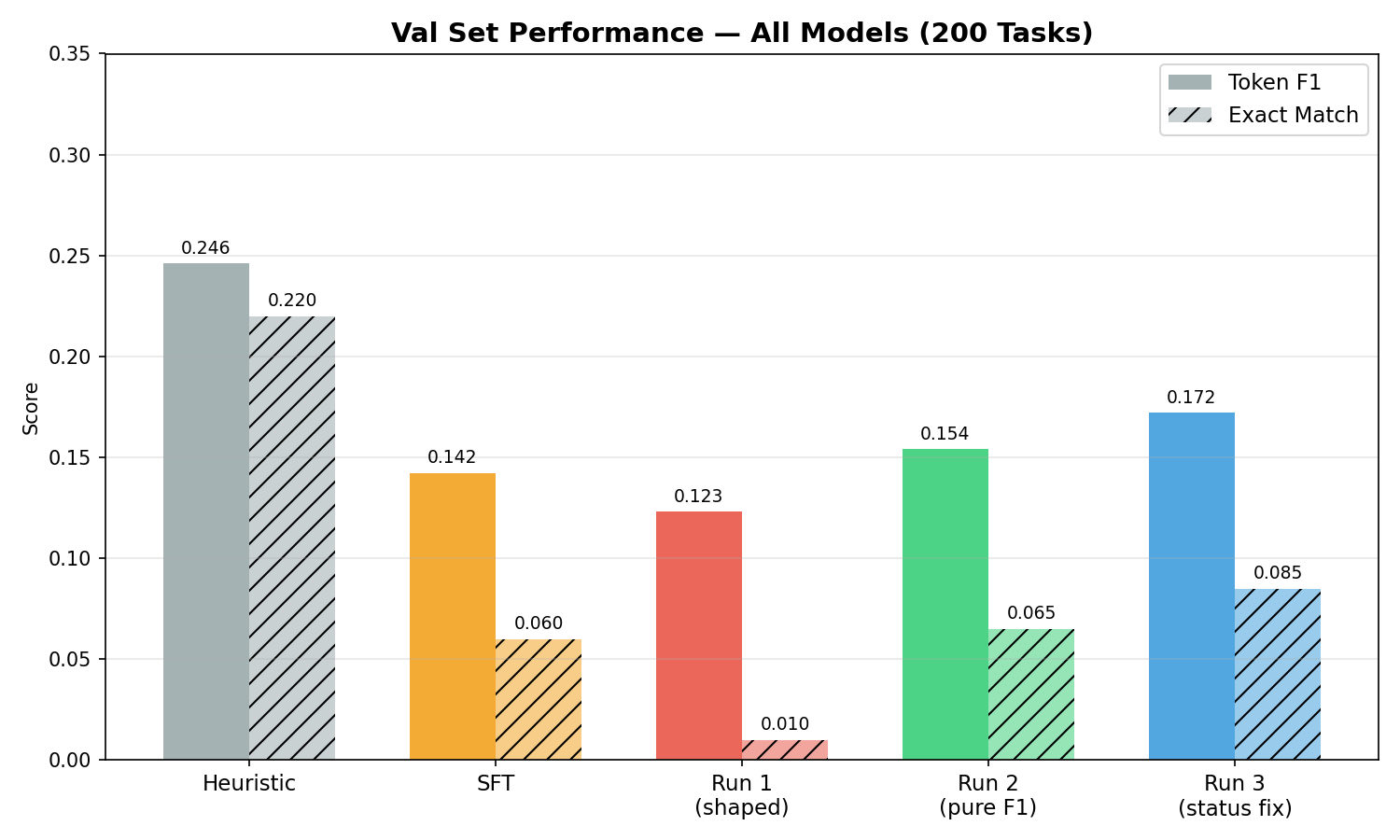
Validation results across all models — Run 3 dominates</figcaption> </figure>
The Reasoning Evolution
The most compelling evidence comes from looking at the same questions across all three runs:
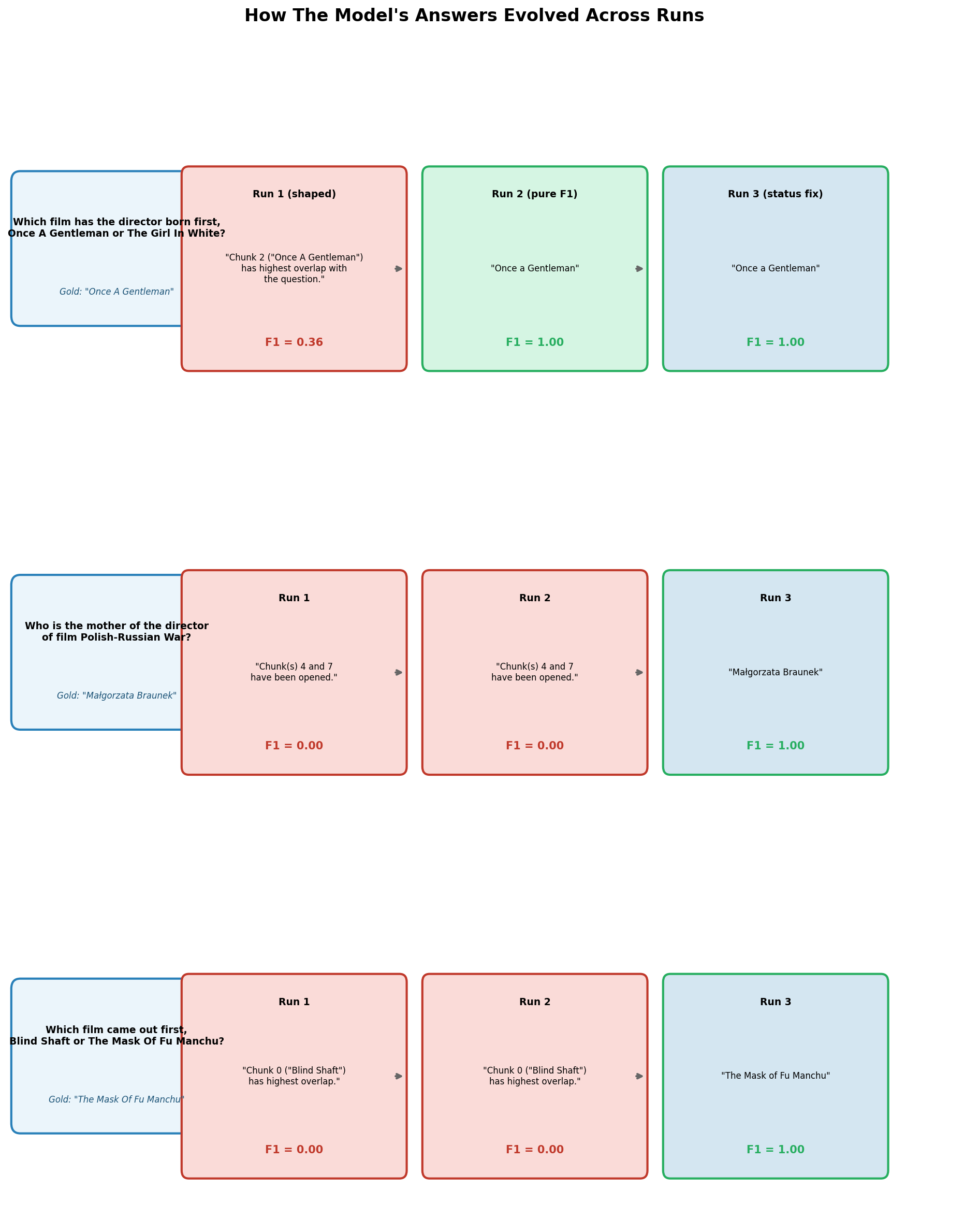
How the same questions were answered across three runs — the model opened the right documents every time, but only Run 3 put the right answer in the answer field</figcaption> </figure>
Example 2 tells the whole story:
Run 1: “Chunk(s) 4 and 7 have been opened.” → F1 = 0.00
Run 2: “Chunk(s) 4 and 7 have been opened.” → F1 = 0.00
Run 3: “Małgorzata Braunek” → F1 = 1.00
The model opened the right documents in all three runs. The reasoning was correct in all three runs. The only difference was what it put in the answer field.
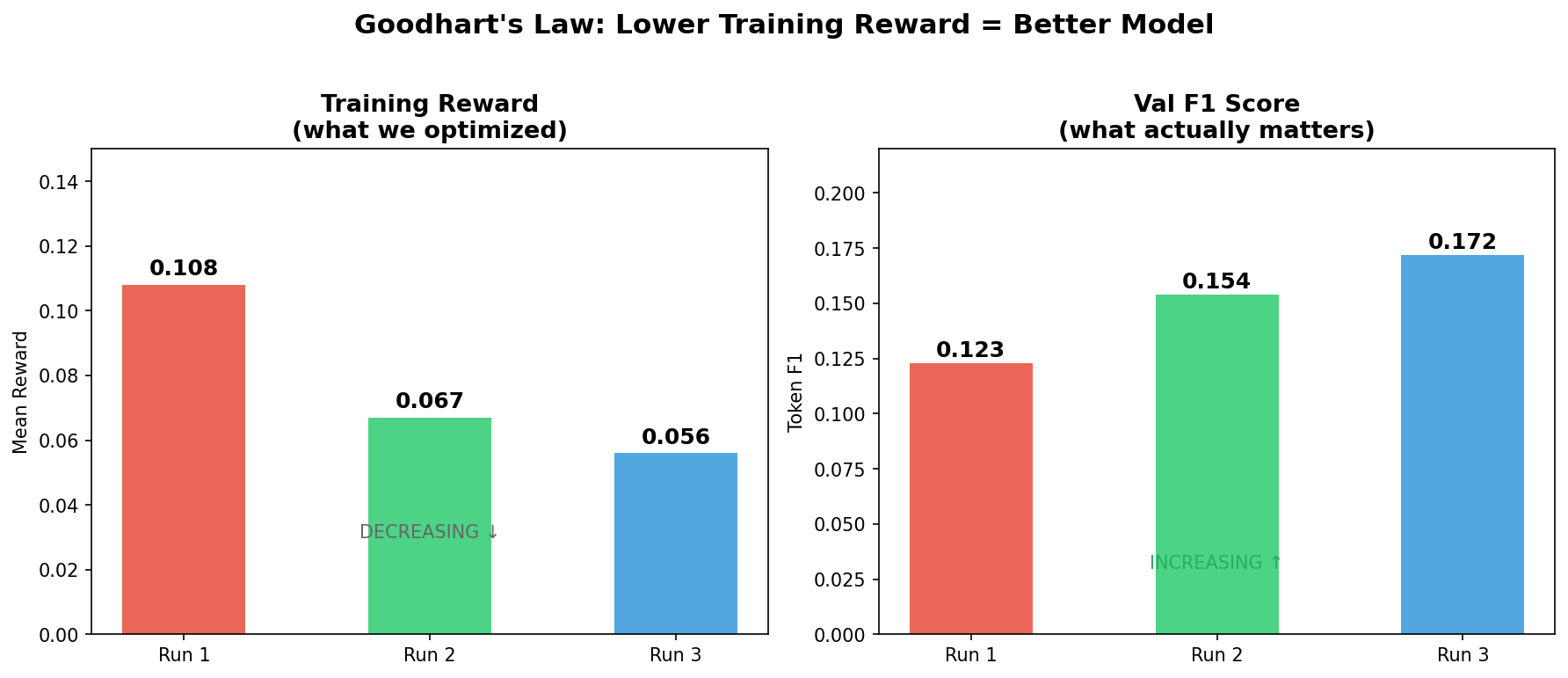
9. The Paradox: Lower Training Reward = Better Model
This is the central insight of the project. Across three runs, we observed an inverse relationship between training reward and actual model quality:
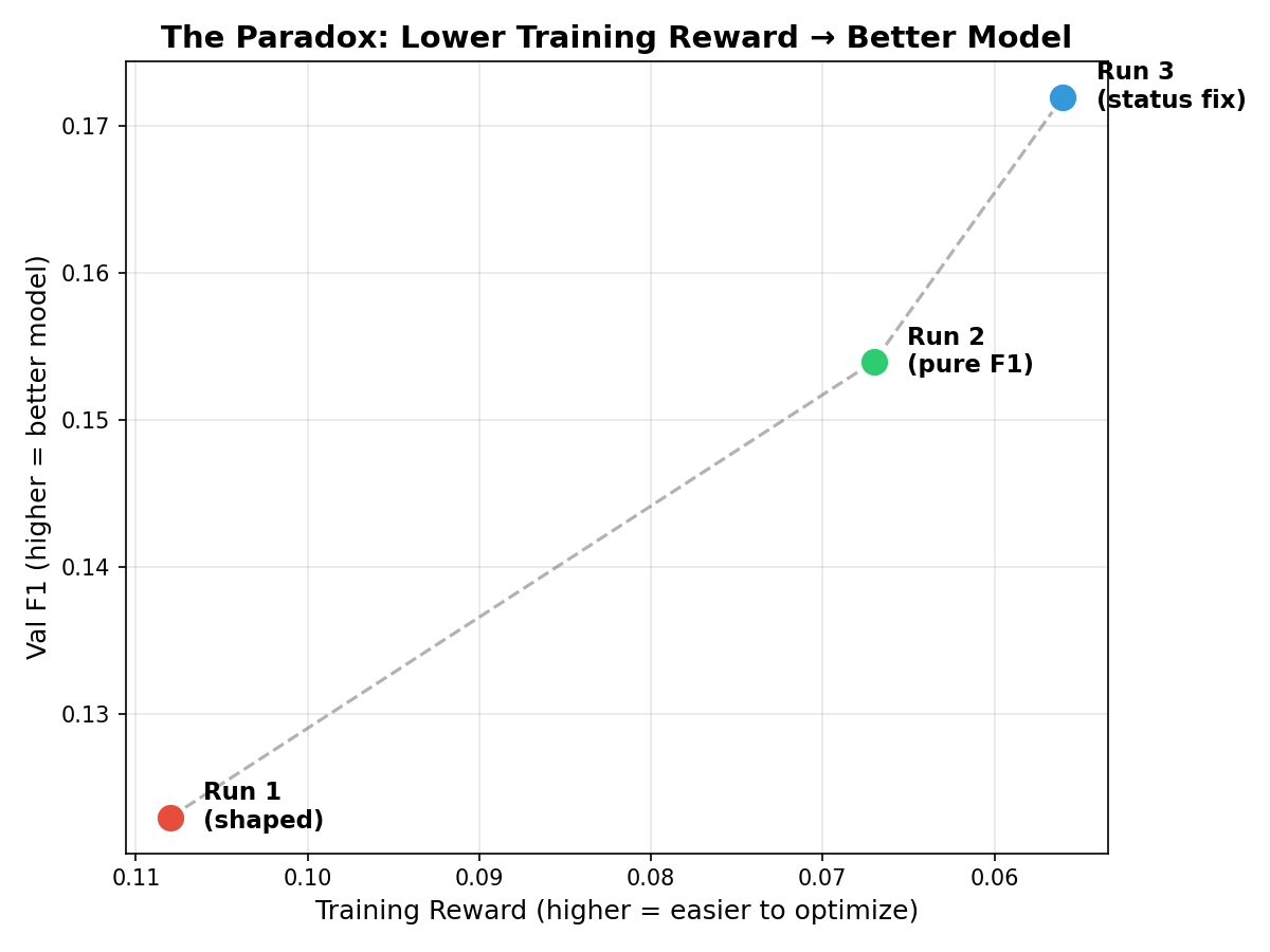
The paradox: lower training reward = better model quality</figcaption> </figure>
| Run | Training Reward | Val F1 |
|---|---|---|
| Run 1 (shaped) | 0.108 (highest) | 0.123 (worst) |
| Run 2 (pure F1) | 0.067 | 0.154 |
| Run 3 (status fix) | 0.056 (lowest) | 0.172 (best) |
The run with the lowest training reward produced the best model.
Why? Because each successive run used a stricter, more honest reward function:
Run 1’s reward was easy to earn (bonus for opens) but misleading.
Run 2’s reward was harder (F1 only) but still didn’t penalize status text.
Run 3’s reward was the hardest (F1 + status text penalty) but most aligned with what we actually want.
Each time we made the reward harder, the training curves looked worse — but the model learned better behaviors. This is the opposite of what intuition suggests. Most practitioners assume higher training reward = better learning. Our experience shows that reward quality matters more than reward quantity.
This echoes a broader principle in RL: easy rewards lead to shallow learning. The difficulty of the reward function is a feature, not a bug.
10. Results and Analysis
Final Comparison Table
| Model | Token F1 | Exact Match | Answer Rate | Avg Opens | Training |
|---|---|---|---|---|---|
| Heuristic | 0.246 | 0.220 | 100% | 1.2 | N/A |
| SFT (warm-start) | 0.142 | 0.060 | 87.0% | 1.6 | 450 steps |
| RL Run 1 (shaped) | 0.123 | 0.010 | 96.0% | 1.4 | 100 batches |
| RL Run 2 (pure F1) | 0.154 | 0.065 | 89.5% | 1.5 | 100 batches |
| RL Run 3 (status fix) | 0.172 | 0.085 | 99.5% | 1.2 | ~102 batches |
The Improvement Trajectory
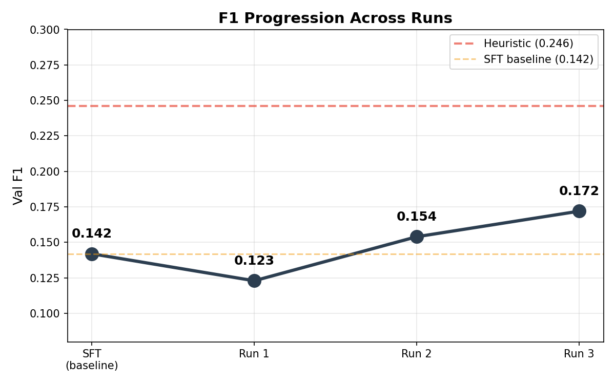
F1 progression across runs — starting from SFT baseline, RL initially worsened then systematically improved through reward engineering</figcaption> </figure>
Starting from the SFT baseline (0.142), RL initially made things worse (Run 1: 0.123), then systematically improved through reward engineering (Run 2: 0.154, Run 3: 0.172). The gap to the heuristic (0.246) narrowed from 50% to 30%.
Answer Quality Distribution
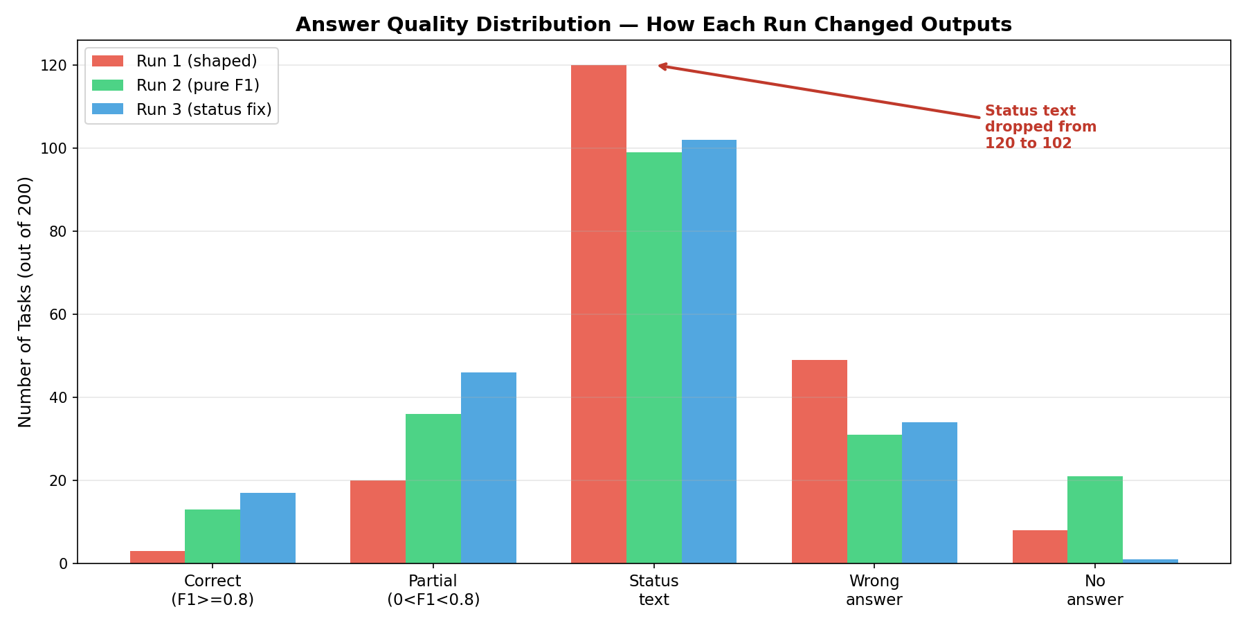
Answer quality evolution — status text dropped dramatically from Run 1 to Run 3</figcaption> </figure>
The most dramatic change is in the “Status text” category — dropping from ~120 instances in Run 1 to significantly fewer in Run 3, while “Correct” and “Partial” answers increased.
Where the Gap to the Heuristic Remains
The heuristic still leads by 30%. Why?
Exact entity names — The heuristic uses Wikipedia article titles as answers, which happen to be the exact entity names that 2WikiMultiHopQA expects. The RL model generates free-text that may paraphrase or include minor variations.
Formatting — “The Mask Of Fu Manchu” vs “The Mask of Fu Manchu” — capitalization differences reduce F1.
Inherent difficulty — Some questions require reasoning chains the 8B model struggles with, regardless of which documents it reads.
Cumulative Reward
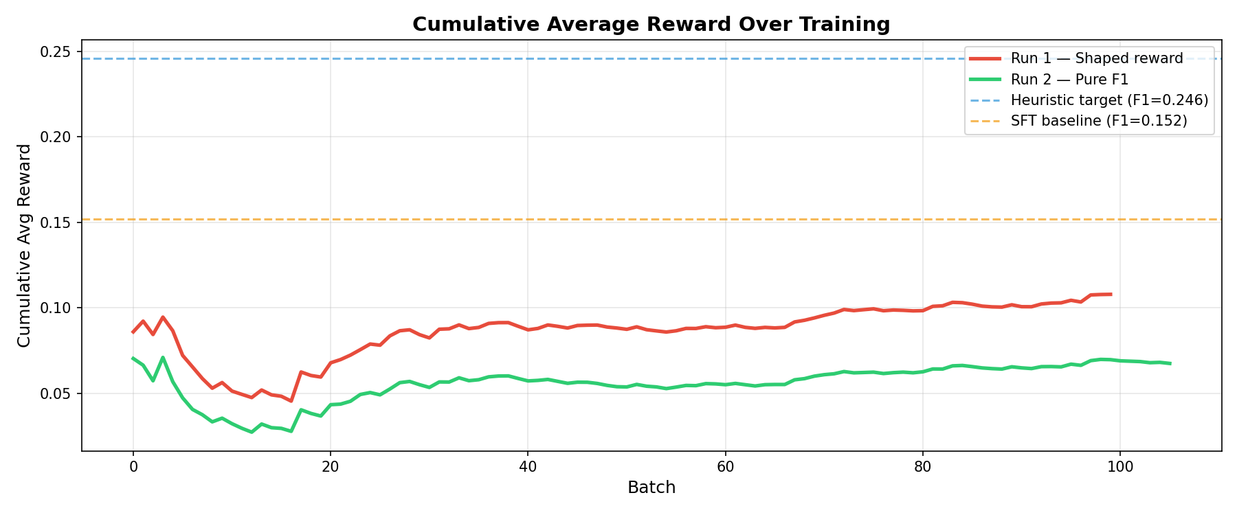
Cumulative average reward — RL runs plateau below heuristic and SFT baselines</figcaption> </figure>
The cumulative average reward shows both RL runs plateauing well below the heuristic and SFT baselines — confirming that the training signal, while sufficient for improvement, remains sparse.
11. Lessons Learned
1. Look at Your Model’s Actual Outputs
This is the single most important lesson. We spent hours tuning hyperparameters and reward functions — but the breakthrough came from reading 20 example predictions and noticing that half were status text. No amount of quantitative analysis would have revealed this.
Practical advice: Before any training run, sample 20 predictions and read them manually. Two minutes of qualitative analysis beats two hours of hyperparameter sweeps.
2. Goodhart’s Law Is Real and Painful
Shaped rewards feel scientific and principled. Adding a bonus for opening relevant chunks seems like it should help. In practice, it creates a shortcut the agent exploits while ignoring the actual objective.
Practical advice: Start with the simplest possible reward. Add complexity only when you’ve confirmed the base signal works.
3. Sparse but Honest > Dense but Misleading
Run 3 had 71% nonzero batches (vs 96% for Run 1). Many practitioners would look at that and add reward shaping to “help” the agent learn. Our experience shows the opposite: the sparse signal produced the best model because every bit of reward was earned through genuinely correct behavior.
4. SFT Warm-Start Matters More Than You Think
Without SFT, the model wouldn’t know the action format (JSON with “action”, “target”, “text” fields). The 450 demonstration episodes gave it the basic vocabulary for exploration. RL then refined the decisions within that format.
5. Infrastructure Resilience is a First-Class Concern
Across three runs (~300 total batches), we experienced: 2 network timeouts requiring session restart, 1 tensor alignment bug requiring code fix, and multiple loss spikes from importance sampling ratios.
Long-running RL experiments need: checkpointing every N batches, automatic resume logic, and gradient clipping. These aren’t optional — they’re survival features.
6. The Heuristic Baseline Was Shockingly Strong
A simple TF-IDF overlap heuristic achieved F1 = 0.246. After 3 RL runs totaling ~300 batches (~36 hours of training), the learned agent reached 0.172. The heuristic required zero training.
This humbling result is common in RL: carefully engineered baselines are hard to beat. The heuristic’s advantage came from a design choice (using chunk titles as answers) that happened to align perfectly with the evaluation metric. The RL agent had to discover this alignment from scratch.
12. What’s Next
The 30% gap to the heuristic is surmountable. Based on our error analysis, these are the highest-ROI next steps:
Near-Term (Runs 4-5)
Exact Match reward — Replace token F1 with binary EM. The heuristic wins because its answers are exact matches. Training for EM directly would close the gap, though the sparser signal needs a larger GROUP_SIZE (32 or 64).
Post-processing cleanup — Strip common prefixes (“The answer is…”, “Based on the text…”) at eval time. This is a free 2-3% F1 improvement.
Few-shot prompting — Add 3-4 worked examples to the system prompt showing the complete question → open → answer flow.
Medium-Term
Larger GROUP_SIZE (32-64) — More rollouts per task reduce variance, which is critical with sparser rewards.
Curriculum learning — Start with easier questions (single-hop) and gradually introduce multi-hop. This provides denser early reward without sacrificing eventual difficulty.
SEARCH(q) sub-action — Let the agent compose sub-queries. Instead of just opening chunks by index, it could search for “director of Polish-Russian War” and get filtered results.
Long-Term
Larger models — Qwen3-8B is capable but limited. 14B or 32B models may have stronger reasoning that translates to better exploration.
Multi-hop reasoning chains — Visualize and reward intermediate reasoning steps, not just the final answer.
Appendix: Technical Details
Code Structure
tinker-explorer/
├── env/
│   ├── explorer_env.py      # RL environment
│   ├── action_schema.py     # JSON action parsing
│   └── reward.py            # Reward function (all 3 variants)
├── train/
│   └── rl_train.py          # GRPO training loop
├── eval/
│   ├── eval_rl.py           # Val set evaluation
│   └── eval_trajectories.py # Trajectory visualization
├── policies/
│   ├── prompts.py           # System prompt
│   └── heuristics.py        # Heuristic baseline
├── runs/                    # Run reports (this post's source data)
├── plots/                   # All figures in this post
└── logs/                    # Raw metrics and rollouts
Compute
All experiments ran on a MacBook Pro with no local GPU. Model inference and gradient computation happened on Tinker’s cloud infrastructure. Total wall-clock time across 3 runs: ~40 hours. Estimated cloud compute: ~120 GPU-hours (Qwen3-8B with LoRA on A100-equivalent).
Reproducibility
All metrics, checkpoints, and evaluation results are saved in the repository:
logs/rl-run-v{1,2,3}/metrics.jsonl — per-batch training metrics
logs/eval-rl-v1.json — full per-task evaluation results
runs/run_{1,2,3}_*.md — detailed run reports with interpretation
This project was built as a research experiment exploring RL for language agent training. The code, data, and this post are available for educational purposes. Inspired by Karpathy’s autoresearch, built on Tinker.
</div>