Designing Reinforcement Learning Environments for Reasoning LLMs
A detailed roadmap and implementation study on building verifier based reinforcement learning environments, synthetic data pipelines, and ReasonRL for reasoning language models.
The Environment Behind Reasoning
Most discussions about reasoning language models start with the optimizer. They ask whether the model was trained with supervised traces, preference optimization, reinforcement learning from human feedback, or verifier based reinforcement learning. Those details matter, but they hide a deeper question: what environment produced the learning signal in the first place?
Reasoning improvement is not only a story about larger models or stronger optimizers. It is also a story about the quality of the training environment. In classic reinforcement learning, this point is obvious. Atari, Go, MuJoCo, Procgen, and procedurally generated worlds define what the agent can observe, what actions it can take, how reward is assigned, and how generalization is measured (Mnih et al., 2015; Cobbe et al., 2020; Dennis et al., 2020). For reasoning LLMs, the environment is less visible, but it is just as important.
A reasoning LLM does not usually interact with a game screen or a robot simulator. Its environment is a synthetic task system. It generates problems, builds prompts, receives model attempts, extracts answers, verifies correctness, assigns rewards, schedules difficulty, and stores trajectories for future training. In that sense, the environment is not a background detail. It is the system that decides what reasoning behavior becomes learnable.
This is especially clear in recent reasoning model work. OpenAI describes o1 as being trained with large scale reinforcement learning to improve chain of thought behavior, while DeepSeek R1 shows that verifier style reinforcement learning can produce strong reasoning behavior even before the usual supervised fine tuning stage is fully relied on (OpenAI, 2024; DeepSeek AI, 2025). The important lesson is not just that reinforcement learning works. The lesson is that reinforcement learning needs a task distribution, a verifier, a reward function, and a curriculum that make reasoning measurable.
The practical question is how to build that loop without becoming an infrastructure lab. This is where newer training platforms matter. Thinking Machines Lab's Tinker separates the research loop from the distributed systems problem: the researcher writes the data, environment, algorithm, and loss, while the platform handles large scale training infrastructure (Thinking Machines Lab, no date). Prime Intellect's Lab takes a related environment first view: a run can drive rollouts through an environment, score trajectories with a rubric, and train a LoRA adapter through its RL stack (Prime Intellect, 2026). These platforms do not remove the need for environment design. They make the environment design more central, because the researcher still has to define the tasks, verifier, rewards, curriculum, and evaluation.
Synthetic data becomes valuable when it is generated and filtered through this kind of environment. Raw generated examples are cheap. Verified synthetic experience is different. It gives the model attempts, failures, rewards, difficulty labels, and successful trajectories. That is the shift this blog is about: from treating reasoning data as static examples to treating reasoning as an interaction loop.
Brief History of RL Environment Design
This section briefly traces RL from MDPs, Bellman equations, TD learning, Q learning, DQN, policy gradients, and PPO to Gym environments, Procgen, curriculum learning, UED, RLHF, and RLVR. The goal is not a textbook history, but the background needed to understand why environments shape reasoning.
Markov Decision Processes
The cleanest starting point for reinforcement learning environment design is the Markov Decision Process. Before there is PPO, Q learning, or verifier based RL, there is a more basic question: what is the decision problem? The Stanford CS237B notes introduce this through sequential decision making, where an agent must choose actions over time while reasoning about future consequences and uncertainty in the environment (Bohg, Pavone and Sadigh, 2025).
In the deterministic version, the system evolves in discrete time. The state at the next step is determined by the current state and the chosen control:
$$x_{k+1} = f_k(x_k, u_k), \qquad k = 0, \ldots, N - 1.$$
Here, $x_k$ is the state, $u_k$ is the control or action, $f_k$ is the transition model, and $N$ is the finite planning horizon. The environment also restricts which actions are allowed from each state:
$$u_k \in U(x_k).$$
This detail matters more than it first appears. An environment is not only a place where actions happen. It defines the action set. A car at an intersection may be allowed to turn left or right, but not drive through a wall. A reasoning LLM may be allowed to produce a final answer, call a verifier, or continue a scratchpad, but each of those choices should be made explicit by the environment design.
The objective is usually written as an additive cost over the trajectory:
$$J(x_0, u_0, \ldots, u_{N-1}) = g_N(x_N) + \sum_{k=0}^{N-1} g_k(x_k, u_k).$$
The terminal cost $g_N(x_N)$ scores where the agent ends up, while the stage cost $g_k(x_k, u_k)$ scores each intermediate decision. The deterministic decision problem is then to find the action sequence that minimizes this total cost:
$$J^*(x_0) = \min_{u_k \in U(x_k),\; k=0,\ldots,N-1} J(x_0, u_0, \ldots, u_{N-1}).$$
In reasoning LLM terms, this is the first useful translation. The prompt is the initial state. Each reasoning step is an action. The scratchpad is the evolving state. The verifier creates the final reward or cost. A long chain of reasoning is not judged only by whether each sentence sounds good, but by whether the sequence reaches a correct final state.
The key idea that makes this tractable is the principle of optimality. If a full sequence of decisions is optimal, then the tail of that sequence should also be optimal from the state it reaches. This turns an impossible brute force search over every full path into a recursive problem over smaller tail problems. Dynamic programming uses this idea by working backward from the terminal state:
$$J_k^*(x_k) = \min_{u_k \in U(x_k)} \left[g_k(x_k, u_k) + J_{k+1}^*(f_k(x_k, u_k))\right].$$
This equation is the conceptual ancestor of much of reinforcement learning. It says that the value of an action is its immediate cost plus the optimal future cost it leads to. When we later talk about Q learning, value functions, or policy optimization, we are still circling this same idea: good actions are good because of the futures they make reachable.
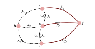
Figure 2.2 captures the intuition. If the optimal paths from $c$, $d$, and $e$ to $f$ are already known, the decision from $b$ does not need to enumerate every possible complete route. It only needs to compare the immediate move to $c$, $d$, or $e$ plus the already known optimal tail cost:
$$\min \{J_{bc} + J_{cf}^*,\; J_{bd} + J_{df}^*,\; J_{be} + J_{ef}^*\}.$$
This is exactly the kind of structure we want in reasoning environments. A reasoning model should not treat each full solution as an isolated string. It should learn which intermediate states make successful completions more likely. A good environment therefore needs to expose not just final answers, but trajectories, partial progress, and the cost or reward structure that connects local reasoning choices to final correctness.
The stochastic version adds uncertainty. Instead of assuming the next state is fully determined, the system includes a disturbance term:
$$x_{k+1} = f_k(x_k, u_k, w_k).$$
The objective then becomes an expected cost under a policy $\pi$, where the policy maps states to actions:
$$J^\pi(x_0) = \mathbb{E}_w \left[g_N(x_N) + \sum_{k=0}^{N-1} g_k(x_k, \pi_k(x_k), w_k)\right].$$
This is closer to language model training. The model is a stochastic policy over text. The same prompt can produce different reasoning traces, some correct and some wrong. Environment design decides how those traces are sampled, scored, filtered, replayed, and converted into learning signal.
Temporal-Difference Learning
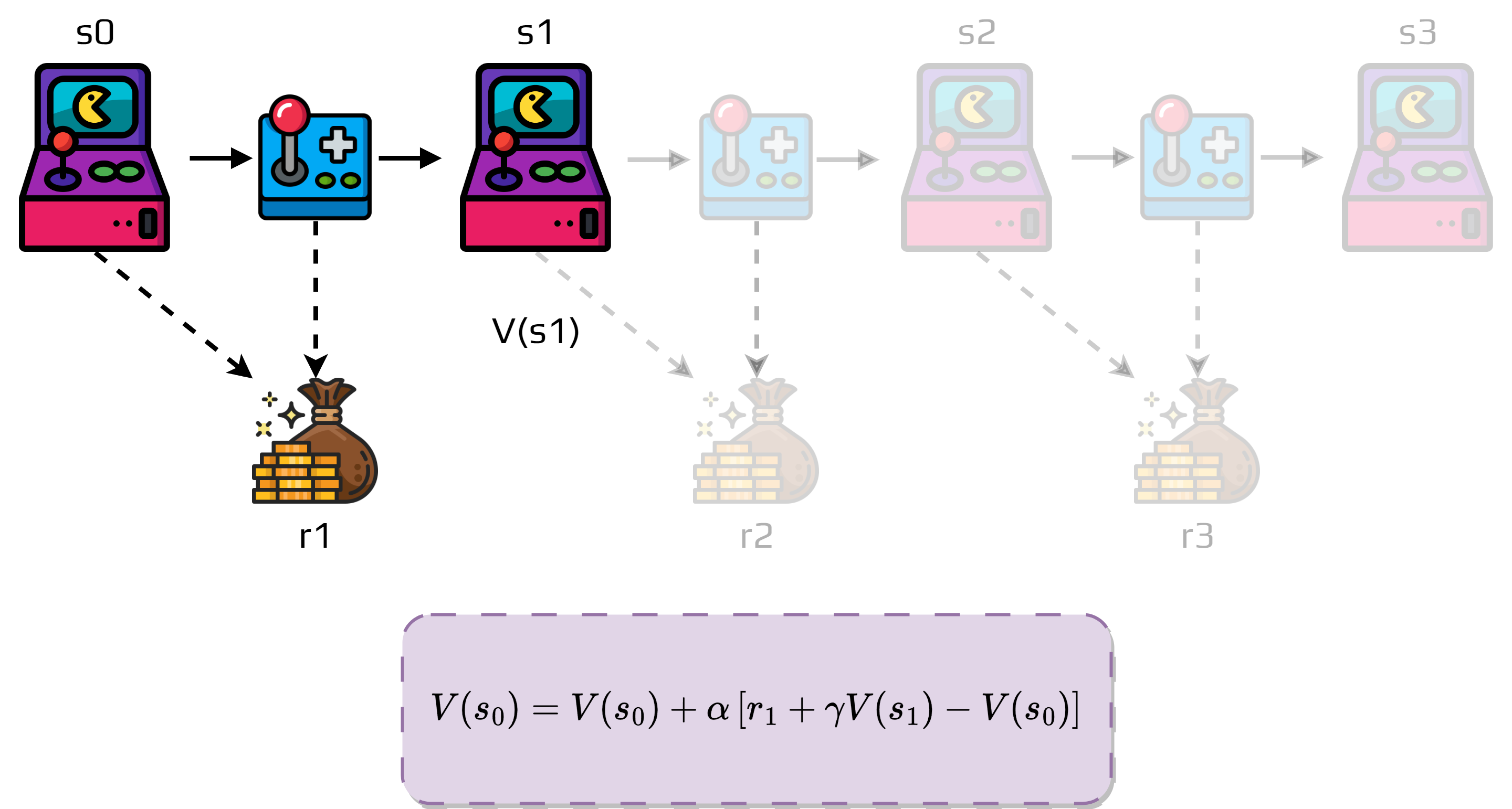
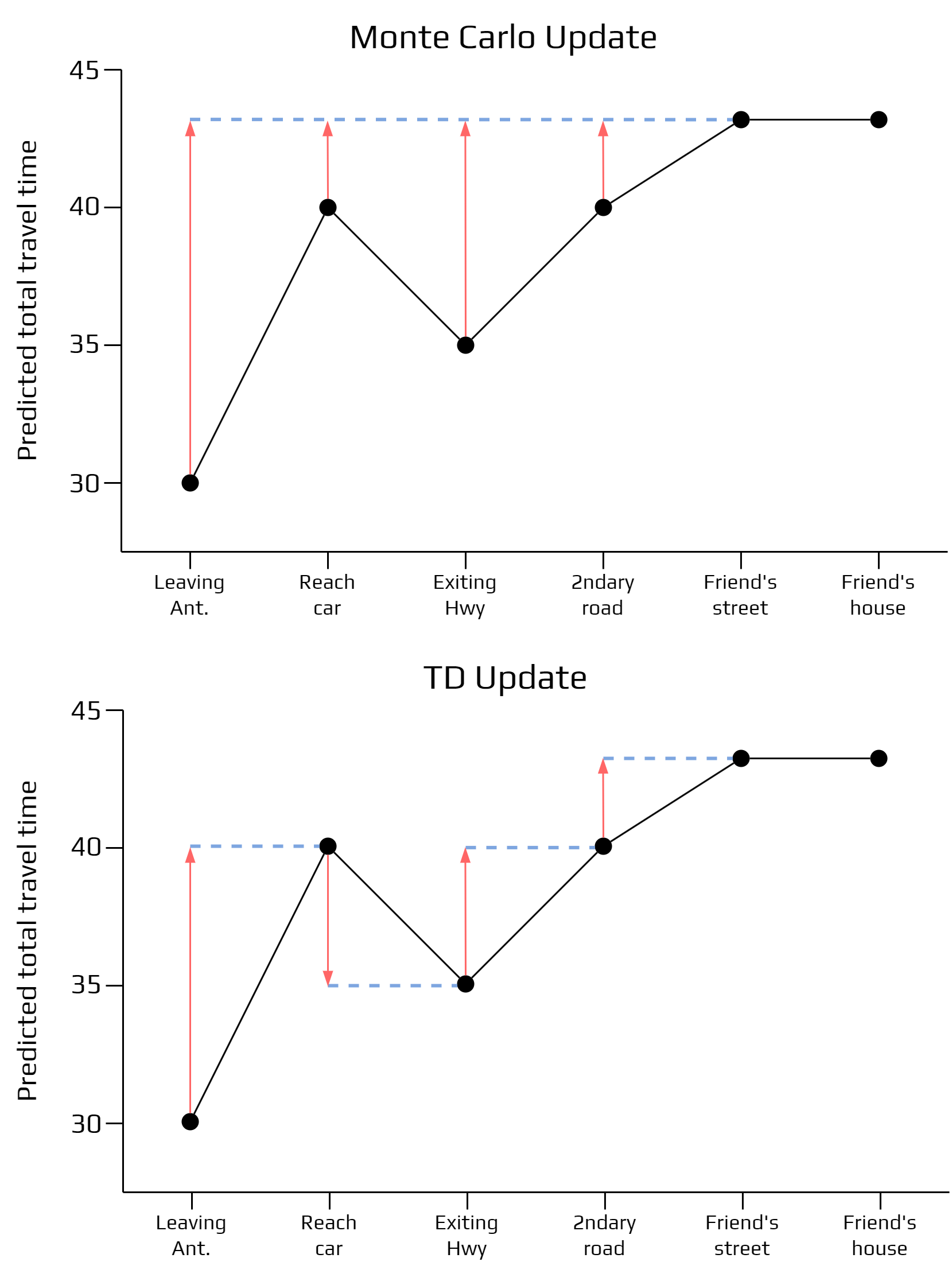
Dynamic programming gives the conceptual foundation, but it assumes we can work with the transition model. Monte Carlo methods move in the opposite direction: they learn from complete sampled episodes, but they must wait until the end of the trajectory before updating. Temporal-Difference learning sits between the two. It learns directly from experience like Monte Carlo, while bootstrapping from the current value estimate like dynamic programming (Delamer, 2024).
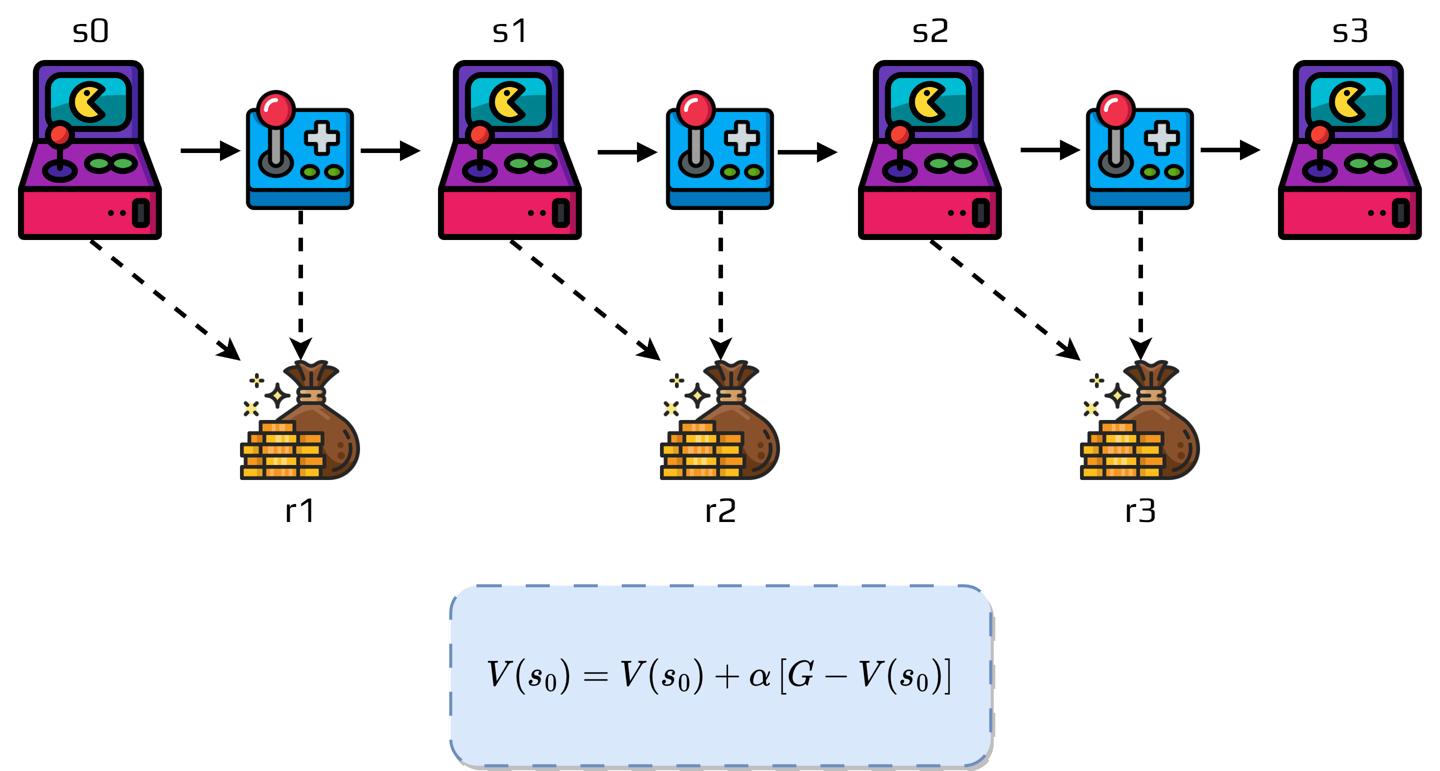
The key TD idea is to update the value of the current state using the reward observed at the next step and the current estimate of the next state's value:
$$V(s_t) \leftarrow V(s_t) + \alpha \left[r_{t+1} + \gamma V(s_{t+1}) - V(s_t)\right].$$
The term inside the brackets is the temporal difference error:
$$\delta_t = r_{t+1} + \gamma V(s_{t+1}) - V(s_t).$$
This error measures the gap between what the model believed about $s_t$ and the improved one step target $r_{t+1} + \gamma V(s_{t+1})$. It is not a final truth. It is a better estimate built from immediate evidence plus the current estimate of the future. That is why TD learning is often described as incremental and online: the agent can update after each transition instead of waiting for the episode to finish.
This distinction matters for reasoning LLMs. If we only reward the final answer, the model gets a sparse signal at the end of a long chain. TD thinking suggests a different design question: can the environment provide intermediate value estimates for reasoning states? A scratchpad state that moves the solution closer to a verified answer should become more valuable; a locally fluent but misleading step should become less valuable. The hard part is building reliable intermediate signals without rewarding superficial reasoning style.


TD learning also leads naturally to action value methods. In SARSA, the update uses the next action actually selected by the current policy:
$$Q(s_t,a_t) \leftarrow Q(s_t,a_t) + \alpha \left[r_{t+1} + \gamma Q(s_{t+1},a_{t+1}) - Q(s_t,a_t)\right].$$
This is on-policy learning: the value update follows the behavior of the policy being learned. Q-learning changes the target by taking the best next action according to the current value estimates:
$$Q(s_t,a_t) \leftarrow Q(s_t,a_t) + \alpha \left[r_{t+1} + \gamma \max_{a'} Q(s_{t+1},a') - Q(s_t,a_t)\right].$$
This is off-policy learning: the model can learn about a greedy target policy even while exploring with another behavior policy. For language models, this distinction foreshadows a major question in reasoning RL: should we train only on the model's own sampled reasoning behavior, or can we learn from trajectories generated by search, rejection sampling, stronger teachers, or older policies? TD learning gives the vocabulary for that question: bootstrapping, temporal error, on-policy updates, and off-policy targets.
Policy-Gradient Reinforcement Learning
Temporal-Difference learning still centers the value estimate. Policy-Gradient Reinforcement Learning turns the focus directly toward the policy. Instead of first learning a table or function that says how good each state or action is, policy-gradient methods parameterize the behavior itself as $\pi_\theta(a \mid s)$ and adjust $\theta$ so that sampled trajectories receive higher expected reward. This makes policy gradients especially important in modern deep RL, where actions may be continuous, high dimensional, or represented by a neural network distribution (Phon-Amnuaisuk, 2018; Sutton and Barto, 2018).
The basic objective is the expected discounted return under the current policy:
$$J(\theta) = \mathbb{E}_{\tau \sim \pi_\theta}\left[\sum_{t=0}^{\infty} \gamma^t r_t\right].$$
The policy-gradient theorem gives a way to differentiate this objective without differentiating through the full environment dynamics:
$$\nabla_\theta J(\theta) = \mathbb{E}_{\pi_\theta}\left[\sum_{t=0}^{\infty} \gamma^t Q^{\pi_\theta}(s_t,a_t)\nabla_\theta \log \pi_\theta(a_t \mid s_t)\right].$$
This equation is one of the reasons policy gradients became central. It says that actions with high downstream value should become more likely, and actions with low downstream value should become less likely. In practice, the $Q$ term is often replaced by a return estimate, a learned critic, or an advantage function:
$$A^{\pi}(s_t,a_t) = Q^{\pi}(s_t,a_t) - V^{\pi}(s_t).$$
The advantage form is useful because it asks a sharper question: was this action better or worse than what the policy normally achieves from this state? For reasoning LLMs, this maps cleanly onto the difference between a sampled reasoning step and the model's expected behavior on that prompt. The training signal should not merely ask whether a final answer was correct. It should ask which sampled decisions increased the probability of getting there.
The earliest actor-only version is REINFORCE, which estimates the gradient from sampled returns. Actor-critic methods add a critic that learns a value function and supplies a lower-variance learning signal. Algorithms such as A2C and PPO belong to this family, with PPO adding a clipped surrogate objective that discourages destructive policy updates (Schulman et al., 2017):
$$L^{\text{CLIP}}(\theta) = \mathbb{E}_t\left[\min\left(r_t(\theta)\hat{A}_t,\; \text{clip}(r_t(\theta), 1 - \epsilon, 1 + \epsilon)\hat{A}_t\right)\right],$$
where
$$r_t(\theta) = \frac{\pi_\theta(a_t \mid s_t)}{\pi_{\theta_{old}}(a_t \mid s_t)}.$$
The reason this matters for reasoning LLMs is stability. A language model policy is extremely high dimensional. If an RL update makes the model much more likely to produce rewarded completions but destroys format following, calibration, or general language behavior, the environment has not produced a better reasoner. It has produced a reward overfit model. PPO-style constraints, KL penalties, and careful batch construction are all attempts to keep the policy improvement step from moving too far at once.
| Family | Main idea | Why it matters here |
|---|---|---|
| REINFORCE | Estimate the gradient from Monte Carlo returns. | Simple but high variance, useful as the conceptual baseline. |
| Actor-critic | Train a policy actor and value critic together. | The critic can reduce variance and estimate intermediate reasoning state value. |
| PPO | Optimize a clipped surrogate objective. | Controls update size, which is crucial for large language policies. |
| Off-policy hybrids | Combine policy-gradient updates with replay or Q-learning style signals. | Relevant when using search traces, rejected samples, or old model rollouts. |
Modern policy-gradient research extends this core idea in many directions. General-utility policy gradients optimize differentiable functions of the state-action occupancy measure $\mu_\pi(s,a)$ rather than only the linear sum of rewards (Kumar et al., 2022; Zhang et al., 2020):
$$J(\theta) = U(\mu_{\pi_\theta}).$$
This matters because reasoning environments may care about more than final reward. They may care about coverage of task types, exploration, information gain, constraint satisfaction, or balanced performance across difficulty buckets. Risk-sensitive policy gradients optimize objectives such as distortion risk measures, making it possible to care about tail behavior rather than only average reward (Vijayan and Prashanth, 2021). Safe policy-gradient work adds probabilistic constraints so the policy can optimize reward while keeping trajectories inside acceptable safety sets (Chen, Subramanian and Paternain, 2022).
There is also a growing line of work on reducing variance, improving exploration, and adapting optimization itself. Weak-derivative estimators offer an alternative to the standard score-function estimator (Bhatt, Koppel and Krishnamurthy, 2020). Hybrid stochastic estimators combine REINFORCE-style unbiased gradients with SARAH-style variance reduction (Pham et al., 2020). Policy-cover guided policy gradient uses an ensemble of policies to improve exploration coverage (Agarwal et al., 2020). Polyak step-size adaptation aims to reduce manual learning-rate tuning (Li et al., 2024).
The most important takeaway for this blog is simple: policy gradients make the policy itself the object of optimization. In reasoning LLMs, that policy is the model distribution over reasoning traces. The environment must therefore define what traces are sampled, how they are scored, how much the update is allowed to move the model, and whether the objective rewards genuine reasoning or only surface behavior. A powerful optimizer cannot repair a poorly designed reasoning environment. It will simply optimize the wrong signal more efficiently.
PPO and GRPO in Deep Reinforcement Learning
Proximal Policy Optimization and Group Relative Policy Optimization are two important descendants of policy-gradient thinking. PPO became a default deep RL baseline because it makes policy optimization practical: it keeps the policy update close to the policy that generated the data, while still allowing multiple epochs of minibatch optimization on the same rollout batch (Schulman et al., 2017). GRPO keeps the proximal update intuition, but replaces the learned value critic with group-relative reward normalization, which is why it became important for large language model post-training and verifier-based reasoning tasks (Shao et al., 2024; DeepSeek AI, 2025).
PPO was introduced as a simpler alternative to Trust Region Policy Optimization. TRPO tries to constrain the policy update using a trust-region constraint, but the implementation is heavier because it involves second-order optimization machinery. PPO turns the same stability instinct into a first-order clipped surrogate objective:
$$L^{\text{CLIP}}(\theta) = \mathbb{E}_t\left[\min\left(r_t(\theta)\hat{A}_t,\; \text{clip}(r_t(\theta), 1 - \epsilon, 1 + \epsilon)\hat{A}_t\right)\right],$$
with the importance sampling ratio
$$r_t(\theta) = \frac{\pi_\theta(a_t \mid s_t)}{\pi_{\theta_{old}}(a_t \mid s_t)}.$$
If the new policy assigns much higher or lower probability to an action than the old policy, the clipped objective limits the benefit of pushing farther in that direction. The effect is conservative policy improvement. PPO can still move the policy, but it discourages the destructive jumps that often destabilize vanilla policy-gradient training.
The standard PPO training loop has two phases. First, run the current policy in the environment and collect trajectories. Second, freeze that batch and run several epochs of minibatch optimization using the clipped objective, an advantage estimate, and often a value-function loss and entropy bonus. This is why PPO is efficient in practice: it decouples sampling from optimization while keeping the policy update close enough to the data-generating policy.
GRPO starts from a similar problem but removes the critic. For each prompt or input, the model samples a group of completions. Each completion receives a scalar reward, often from a verifier. Instead of estimating an advantage with a value model, GRPO normalizes rewards inside the group:
$$A_i = \frac{r_i - \mu_G}{\sigma_G + \delta},$$
where $r_i$ is the reward for rollout $i$, $\mu_G$ is the group mean, $\sigma_G$ is the group standard deviation, and $\delta$ is a small constant for numerical stability. A completion is therefore not judged in isolation. It is judged relative to the other completions sampled for the same task.
The GRPO objective keeps the PPO-style clipped update but uses group-relative advantages and often includes a KL penalty against a reference model:
$$L_{\text{GRPO}}(\theta) = \frac{1}{|G|}\sum_{i=1}^{|G|}\sum_{t=1}^{T}\min\left(w_t^{(i)}A_i,\; \text{clip}(w_t^{(i)}, \epsilon_{low}, \epsilon_{high})A_i\right) - \beta D_{KL}(\pi_\theta \Vert \pi_{ref}),$$
where
$$w_t^{(i)} = \frac{\pi_\theta(y_t^{(i)} \mid x, y_{1:t-1}^{(i)})}{\pi_{\theta_{old}}(y_t^{(i)} \mid x, y_{1:t-1}^{(i)})}.$$
For reasoning LLMs, this is attractive because the critic is expensive. A value model for every token in every long chain of thought consumes memory, compute, and engineering complexity. GRPO avoids that critic by using the group itself as the baseline. If four or eight solutions are sampled for the same math problem, the correct or high-reward solutions become positive examples relative to the weaker ones. This is a natural fit for tasks with automatic verifiers.
| Method | Advantage source | Strength | Trade-off |
|---|---|---|---|
| PPO | Usually a learned critic plus GAE. | Stable, general, widely tested in deep RL. | Requires value model training and careful tuning. |
| GRPO | Group-normalized empirical rewards. | Critic-free and efficient for verifier-scored LLM rollouts. | Needs multiple samples per prompt and reliable rewards. |
| TIC-GRPO | Group rewards with trajectory-level importance correction. | Addresses bias from token-level stale-policy ratios. | Newer and less established than PPO. |
Recent work has sharpened the theory. Pang and Jin argue that standard GRPO estimates the gradient at the old policy rather than exactly at the current policy because the sampled trajectories are stale, then propose trajectory-level importance corrected GRPO, or TIC-GRPO, to use a full-trajectory probability ratio (Pang and Jin, 2025):
$$L_{\text{TIC-GRPO}}(\theta) = \frac{1}{|G|}\sum_{i=1}^{|G|}\min\left(w_i' A_i,\; \text{clip}(w_i', \epsilon)A_i\right) - \beta D_{KL}(\pi_\theta \Vert \pi_{ref}).$$
Another line of work studies on-policy and off-policy GRPO. Off-policy GRPO is especially relevant for large-scale LLM training systems because rollouts may be generated by slightly older policies or remote inference servers, then reused for training. Mroueh et al. show that off-policy GRPO can match or outperform on-policy variants in RL with verifiable rewards, which matters when sampling is expensive and communication costs are high (Mroueh et al., 2025).
There is also a contrastive interpretation. The paper It Takes Two: Your GRPO Is Secretly DPO argues that, with a minimal group of two rollouts, GRPO resembles a contrastive preference-learning objective: one completion is relatively better, the other relatively worse, and the learning signal comes from their difference (Wu et al., 2025). This gives a useful mental model for LLM reasoning: GRPO is not only optimizing absolute reward; it is asking the model to prefer the better reasoning trace among alternatives.
The practical lesson is that PPO and GRPO answer different engineering needs. PPO is the robust baseline for deep RL when a critic is affordable and stable value estimation is possible. GRPO is attractive when the environment can generate several rollouts per prompt and score them with a verifier, but a token-level critic would be costly. In reasoning LLMs, this pushes the burden back onto the environment: group sampling, verifier quality, reward normalization, KL control, and prompt difficulty all determine whether GRPO produces genuine reasoning improvement or just relative reward hacking.
Unsupervised Environment Design
Unsupervised Environment Design asks a different question from PPO or GRPO. Instead of asking how to optimize a policy inside a fixed environment, it asks how the training environments themselves should be generated. The goal is to expose the agent to enough complexity, variability, and learnable difficulty that it becomes robust rather than overfit to one narrow task distribution (Dennis et al., 2020; Jiang, Grefenstette and Rocktaschel, 2021; Parker Holder et al., 2022).
A useful first distinction is between a state and an environment. In chess, a state is a particular board configuration. The environment is the broader game setup: legal moves, transition rules, opponent behavior, time controls, reward structure, and any variants we choose to train on. So chess can be treated as one environment with many states, but we can also define a family of related environments by changing the opponent, opening distribution, board size, partial observability, or reward design. The environment is the setup condition; the state is what the agent currently observes inside that setup.
In video games, different environments might mean different levels, maps, enemy placements, visual themes, or game modes. In robotics, they might mean different objects to grasp, surfaces to walk on, lighting conditions, masses, friction values, or obstacle layouts. In finance, they might mean different market regimes such as bull markets, bear markets, changing interest rates, asset classes, or risk constraints. The common idea is that the environment has free parameters that shape the agent's experience.
UED is often formalized with an underspecified partially observable Markov decision process, or UPOMDP. The normal POMDP is not enough because the environment itself has free parameters. We therefore introduce a parameter space $\Theta$, where each $\theta \in \Theta$ defines a possible setting of the environment. The transition function can be written as:
$$T_M : S \times A \times \Theta \rightarrow \Delta(S).$$
This means the next-state distribution depends not only on the current state and action, but also on the environment parameter $\theta$. A sequence of environment parameters creates a particular training environment or curriculum. For example, in a warehouse robot simulation, $\theta$ might specify object positions, object shapes, stacking patterns, bin geometry, lighting, friction, or sensor noise. The robot state captures what is currently observed, but $\theta$ controls the conditions that generated the episode.
To generate environments systematically, UED defines an environment policy. One way to write this is:
$$\Lambda : \Pi \rightarrow \Delta(\Theta^T),$$
where $\Pi$ is the set of possible agent policies and $\Theta^T$ is the set of possible sequences of environment parameters across an episode. In plain language, the environment designer looks at the current agent and chooses what kinds of worlds, tasks, levels, or parameter settings the agent should train on next.
PAIRED is an important example of this idea. It trains an adversarial environment generator to create tasks that expose regret: environments where a protagonist agent fails but an antagonist or stronger policy can succeed (Dennis et al., 2020). Prioritized Level Replay then stores and replays levels that are useful for learning, rather than treating every sampled level equally (Jiang, Grefenstette and Rocktaschel, 2021). ACCEL extends the idea by evolving curricula around the frontier of the agent's competence (Parker Holder et al., 2022).
For reasoning LLMs, UED becomes very natural. The environment parameters are no longer object positions or game maps. They are problem templates, number ranges, distractor density, proof length, code edge cases, verifier strictness, and difficulty schedules. A good reasoning environment should not merely generate random problems. It should generate problems that are solvable, diverse, hard enough to teach something, and different enough from the training distribution to measure generalization.
This is where synthetic data becomes an environment-design problem. If we generate easy problems forever, the model memorizes shallow patterns. If we generate impossible problems, the reward becomes noise. UED suggests the middle path: create a task distribution that moves with the learner, exposes failures, and keeps the model near the edge of its current ability. That is exactly the kind of curriculum a reasoning LLM needs.
Why the Environment Defines What Can Be Learned
The history points to one argument: algorithms matter, but the environment defines the learning problem. DQN, PPO, GRPO, TD learning, and UED all optimize behavior, but behavior can only improve relative to the states, actions, transitions, rewards, and task distribution the environment exposes. A weak environment produces a weak learning signal, even with a strong optimizer.
The standard MDP summary is:
$$\text{MDP} = (S, A, P, R, \gamma).$$
| MDP term | Classical meaning | Reasoning LLM meaning |
|---|---|---|
| $S$ | State space. | Prompt plus reasoning context, scratchpad, and previous steps. |
| $A$ | Action space. | Generated reasoning step, tool-free answer, or final response. |
| $P$ | Transition function. | Update to the reasoning trace after the model writes the next step. |
| $R$ | Reward function. | Verifier score, test pass rate, symbolic check, or answer correctness. |
| $\gamma$ | Discount factor. | How much future correctness matters relative to local reasoning moves. |
For a reasoning model, one episode can be written as:
$$s_0 = x, \qquad a_t \sim \pi_\theta(\cdot \mid s_t), \qquad s_{t+1} = P(s_t, a_t), \qquad r_t = R(s_t, a_t).$$
At the end, a verifier assigns the most important reward:
$$R(x, y) = \mathbf{1}[\text{Verifier}(x, y) = \text{correct}].$$
A minimal reasoning environment loop can be described as:
for task in task_generator:
    state = build_prompt(task)
    trace = []

    while not done:
        action = policy.sample(state)
        trace.append(action)
        state = update_reasoning_state(state, action)
        done = is_final_answer(action) or budget_exhausted(state)

    reward = verifier.score(task, trace)
    store_trajectory(task, trace, reward)
And the same idea can be made concrete with a small Python skeleton:
from dataclasses import dataclass


@dataclass
class ReasoningState:
    prompt: str
    scratchpad: list[str]
    step_budget: int


class ReasoningMDP:
    def __init__(self, task_generator, verifier, gamma: float = 1.0):
        self.task_generator = task_generator
        self.verifier = verifier
        self.gamma = gamma

    def reset(self) -> ReasoningState:
        self.task = self.task_generator.sample()
        return ReasoningState(
  prompt=self.task["prompt"],
  scratchpad=[],
  step_budget=self.task.get("step_budget", 8),
        )

    def transition(self, state: ReasoningState, action: str) -> ReasoningState:
        return ReasoningState(
  prompt=state.prompt,
  scratchpad=[*state.scratchpad, action],
  step_budget=state.step_budget - 1,
        )

    def reward(self, state: ReasoningState, action: str) -> float:
        if "final answer:" not in action.lower():
  return 0.0
        return float(self.verifier.is_correct(self.task, state.scratchpad + [action]))

    def done(self, state: ReasoningState, action: str) -> bool:
        return state.step_budget <= 0 or "final answer:" in action.lower()

    def step(self, state: ReasoningState, action: str):
        next_state = self.transition(state, action)
        reward = self.reward(state, action)
        done = self.done(next_state, action)
        return next_state, reward, done
This is deliberately small, but it captures the core idea. The model is not simply fine tuned on examples. It acts inside a defined environment. The environment decides what counts as a state, what actions are allowed, how traces evolve, how answers are verified, and what reward is returned. That is why environment design is the real foundation for RL on reasoning LLMs.
What Is an RL Environment for a Reasoning LLM?
The main lesson from RL history is that progress has always depended on environment structure. Algorithms matter, but the environment defines what the agent can observe, what it can do, how it receives feedback, and therefore what it can learn.
The classical abstraction is:
$$\text{MDP} = (S, A, P, R, \gamma).$$
Here, $S$ is the state space, $A$ is the action space, $P$ is the transition function, $R$ is the reward function, and $\gamma$ is the discount factor. For a reasoning LLM, this maps naturally into a text-based environment: $S$ is the prompt plus reasoning context, $A$ is a generated reasoning step or final answer, $P$ is the update to the reasoning trace, $R$ is the verifier score, and $\gamma$ controls how much future correctness matters.
state = prompt + reasoning_context

while not done:
    action = model.generate_next_step(state)
    state = update_reasoning_trace(state, action)
    reward = verifier.score(state, action)
    done = final_answer_submitted or step_budget_exhausted

store(task, trace, reward)
This is the core shift: the LLM is not just trained on examples. It acts inside a designed environment where tasks are sampled, reasoning traces evolve, answers are verified, and rewards become learning signals.
ReasonEnv: The Components of a Reasoning Environment
A reasoning environment is not just a prompt template. It is a full system around the model. A useful definition is:
$$\text{ReasonEnv} = (\text{TaskGenerator}, \text{StateBuilder}, \pi_\theta, \text{Verifier}, R, \text{Curriculum}, \text{Logger}).$$
Each component has a specific job. The task generator creates problems. The state builder turns a task into a prompt and reasoning context. The policy $\pi_\theta$ is the model. The verifier checks the answer or trace. The reward function turns verification into a scalar signal. The curriculum decides what difficulty comes next. The logger stores trajectories so the system can learn from both success and failure.
The episode loop looks like this:
task = task_generator.sample(difficulty)
state = state_builder.build(task)
trace = []

while not terminated:
    action = policy.generate(state)
    trace.append(action)
    state = transition(state, action)
    terminated = stop_condition(state, action)

verifier_result = verifier.check(task, trace)
reward = reward_function(verifier_result, trace)
logger.write(task, trace, reward, verifier_result)
curriculum.update(task, reward)
This makes the environment concrete. The model does not merely output text into a dataset. It takes actions inside a loop, and the loop decides what feedback is meaningful.
State, Action, Transition, Reward, Termination
The state can include the original prompt, task type, difficulty level, scratchpad, previous reasoning steps, remaining step budget, and optional verifier feedback. The action can be a token, a reasoning step, or a full solution. For a first implementation, full-solution actions are easiest; step-level actions become useful later when we want process rewards.
For full-solution training, the transition is simple:
$$s_0 = x, \qquad a_0 = y, \qquad s_1 = (x, y, \text{Verifier}(x,y)).$$
For step-level training, the transition is incremental:
$$s_{t+1} = s_t \oplus a_t,$$
where $\oplus$ means appending the new reasoning step to the trace. A simple binary verifier reward can be written as:
$$R(x,y) = \begin{cases}1, & \text{if } \text{Verifier}(x,y)=\text{correct},\\0, & \text{otherwise.}\end{cases}$$
A shaped reward can add format and efficiency terms:
$$R = R_{\text{correct}} + \lambda_f R_{\text{format}} - \lambda_l \text{length}(y).$$
But this should be used carefully. If the reward is too shaped, the model may learn to optimize the style of reasoning rather than correctness. For reasoning LLMs, reward design is part of environment design.
Designing the Right Environment
A good reasoning RL environment is not just a prompt collection. It must generate tasks, verify answers, control difficulty, and expose enough variation that the model learns general reasoning strategies rather than memorizing templates. The paper Reasoning Gym: Reasoning Environments for Reinforcement Learning with Verifiable Rewards is useful here because it treats reasoning environments as the central object of RLVR training, not as an afterthought (Stojanovski et al., 2025).
The paper introduces Reasoning Gym, a library of more than 100 procedurally generated reasoning environments with automatic verifiers. These environments cover algebra, arithmetic, computation, cognition, geometry, graph theory, logic, and games. Its purpose is directly connected to this blog section: it shows how to design environments where reasoning tasks are not fixed examples, but generators with adjustable complexity and verifiable rewards.
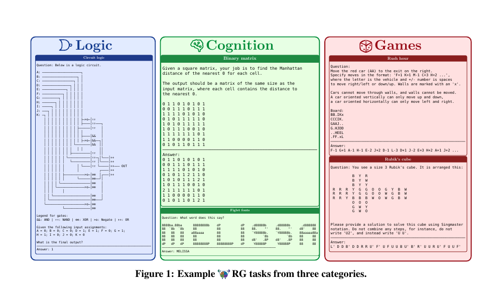
The design principles in the paper are especially important. First, every task should be algorithmically verifiable, meaning no human judgment is needed to assign reward. Second, the solution space should be large enough that the model must learn general strategies rather than exploit a narrow template. Third, the environment should support parametric difficulty control, so the same task family can become easier or harder by changing variables such as graph size, polynomial degree, word length, grid size, number range, or constraint depth.
In environment terms, this means each task family should expose parameters:
$$\theta = (\theta_{difficulty}, \theta_{structure}, \theta_{style}).$$
Difficulty parameters control complexity. Structural parameters control the shape of the reasoning problem. Stylistic parameters vary presentation without changing the underlying skill. This matters because a reasoning model should be tested on the skill, not only on one surface form of the prompt.
task = generator.sample(
    difficulty={"num_steps": 5, "constraint_depth": 3},
    structure={"task_type": "logic_grid"},
    style={"variable_names": "randomized"}
)

answer = model.solve(task.prompt)
reward = verifier.check(task, answer)
The paper also gives a concrete curriculum lesson. In their curriculum RLVR experiments, models trained with progressively increasing difficulty were compared against models trained by sampling uniformly from all difficulty levels. The curriculum setup increased difficulty after the model exceeded a performance threshold, creating a learning path instead of throwing the full distribution at the model immediately.
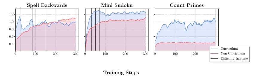
For this blog, the lesson is simple: a good environment should not only ask questions. It should let us control and observe the learning process. We should know which parameter made a task hard, whether the verifier is reliable, whether the model is learning the intended skill, and whether performance transfers to held-out task variants. That is what separates a useful RL environment from a pile of synthetic prompts.
Choosing the Right RL Algorithm
Once the environment is defined, the optimizer is no longer a matter of taste. The algorithm should match the shape of the environment: how rewards arrive, whether the verifier is reliable, whether rollouts are expensive, whether a critic is affordable, and whether the policy starts from a base model or an already aligned model. This is why algorithm selection should come after environment design, not before it.
A useful way to write the choice is:
$$\mathcal{A}^{*} = f(\mathcal{E}, R, \mathcal{S}, \mathcal{A}, D, \pi_0, C),$$
where $\mathcal{E}$ is the environment family, $R$ is the reward or verifier, $\mathcal{S}$ is the state representation, $\mathcal{A}$ is the action representation, $D$ is the available data, $\pi_0$ is the initialized policy, and $C$ is the compute budget. In classical RL, this means asking whether the environment is simulated or real, whether actions are discrete or continuous, whether experience is cheap or expensive, and whether stability or sample efficiency matters more (Bongratz et al., 2024). In reasoning LLMs, the same idea becomes: can I generate multiple answers per prompt, can I verify them, can I afford a value model, and does the model already know how to produce usable reasoning?
| Environment condition | Algorithmic direction | Reason |
|---|---|---|
| Verifier gives a final score and multiple rollouts per prompt are cheap. | GRPO or another critic-free relative policy method. | The group supplies a local baseline, so the model learns from relative success without training a separate critic. |
| A critic is affordable and stable value estimation is possible. | PPO or actor-critic policy optimization. | The critic can reduce variance, while clipped policy updates keep optimization from moving too far at once. |
| Rewards are sparse, binary, or highly skewed. | Use advantage normalization and careful reward scaling. | Raw reward differences can be too noisy. Group means and batch-level standard deviations can make the learning signal more stable (Liu et al., 2025). |
| The model is a base model that does not reliably follow the answer format. | Start with supervised fine-tuning or a warm-start policy, then apply RL. | RL is better at improving a behavior that already exists than inventing a full reasoning format from scratch. |
| The model is already aligned and produces long structured answers. | Prefer conservative PPO or GRPO settings, sequence-level aggregation, and tight evaluation. | Large updates can damage useful structure. The best trick for a base model may not help an aligned model. |
| Outputs become repetitive, truncated, or too long. | Add length-aware filtering or overlong masking. | This can improve short and medium reasoning tasks, but it may be less useful for genuinely long-tail reasoning tasks. |
| Experience comes from old policies, replay buffers, or search traces. | Use off-policy correction, filtering, or keep updates close to the sampling policy. | The farther the data distribution is from the current model, the easier it is to optimize the wrong objective. |
The first split is model-free versus model-based RL. If the environment dynamics are known or can be learned accurately, model-based methods can use planning, simulated rollouts, or learned transition models. If the environment is mostly a verifier over generated language, model-free policy optimization is usually the more direct starting point. For a reasoning LLM, the transition function is often the model extending its own trace, so the practical model of the environment is the task generator plus verifier rather than a physics simulator.
The second split is value-based, policy-based, or actor-critic. Value-based methods such as Q-learning are natural when the action space is small enough to compare actions. That assumption breaks quickly for LLMs because an action may be a token, a reasoning step, or a full answer drawn from a massive vocabulary. Policy-gradient methods fit better because they directly update the probability of sampled text. Actor-critic methods, especially PPO, add a value model to reduce variance. Critic-free methods, especially GRPO-style training, trade the value model for group comparisons among sampled answers.
For reasoning LLMs, the choice between PPO and GRPO should be made from the environment outward. PPO is attractive when we can estimate values and want a stable general baseline. GRPO is attractive when each prompt can produce a group of candidate solutions and the verifier can score them. The group mean acts like a prompt-local baseline:
$$A_i = \frac{r_i - \mu_G}{\sigma_G + \delta}.$$
This is powerful because many reasoning rewards are sparse. If eight completions are sampled for the same math problem, the raw reward may only say correct or incorrect. The group comparison turns that into a usable learning signal: increase the probability of the completion that solved this prompt and decrease the probability of the alternatives.
However, this also creates a design trap. If every completion in the group is wrong, the group gives weak signal. If every completion is correct, it also gives weak signal. That means task difficulty and dynamic sampling matter as much as the optimizer. A good environment should keep the model in the learning band, where some rollouts succeed and some fail. This is the algorithmic version of curriculum design.
for prompt in task_batch:
    rollouts = sample(policy, prompt, n=group_size)
    rewards = [verifier(prompt, y) for y in rollouts]

    if all_same(rewards):
        maybe_resample_or_change_difficulty(prompt)
        continue

    advantages = normalize_within_group(rewards)
    update_policy_with_clipped_objective(policy, rollouts, advantages)
The third split is on-policy versus off-policy. On-policy methods train on data sampled from the current policy, which is cleaner but expensive. Off-policy methods reuse old data, which is cheaper but more fragile. In LLM reasoning, old traces may come from a previous checkpoint, a stronger teacher, rejection sampling, beam search, or Monte Carlo tree search. These traces are valuable, but they are not neutral. They come from another distribution. If we train on them directly, the model may learn the behavior of the data generator rather than improve its own policy.
One practical rule is to separate three data roles: supervised warm start, exploration data, and policy-gradient data. Supervised warm start teaches format and basic competence. Exploration data discovers candidate solutions and failure modes. Policy-gradient data should stay close enough to the current policy that the update still means something.
def choose_algorithm(env):
    if not env.has_verifier:
        return "SFT, preference optimization, or human feedback before RL"

    if env.action_space == "small_discrete":
        return "Q-learning or another value-based method"

    if env.can_sample_groups and env.critic_is_expensive:
        return "GRPO-style critic-free policy optimization"

    if env.can_train_critic and env.needs_stability:
        return "PPO or another actor-critic method"

    if env.uses_old_traces:
        return "off-policy correction, filtering, or supervised warm start"

    return "start with PPO as the baseline, then simplify or specialize"
The recent RL-for-reasoning literature also makes one thing clear: there is no universal trick. Normalization, clipping, token-level loss aggregation, sequence-level loss aggregation, and overlong filtering all interact with model initialization, reward scale, prompt difficulty, and answer length (Liu et al., 2025). For example, token-level aggregation can help base models because it gives each generated token a clearer contribution to the update. But for already aligned models, sequence-level aggregation may preserve the structure of high-quality responses better. Similarly, increasing the upper clipping bound can promote exploration in strong aligned models, but it can also make updates too aggressive if the environment is noisy.
| LLM reasoning choice | When it helps | What to watch |
|---|---|---|
| Group-level normalization | Verifier rewards are sparse and several answers are sampled per prompt. | Groups with all correct or all wrong answers give little contrast. |
| Batch-level standard deviation | Reward scale is large or unstable across prompts. | Can hide prompt-specific difficulty if used without a local mean. |
| Higher clip range | The initialized model is strong and needs room to explore better reasoning paths. | Too much freedom can amplify reward hacking or formatting shortcuts. |
| Token-level loss aggregation | Base models need dense pressure across long completions. | May be less helpful for aligned models with already stable reasoning style. |
| Overlong filtering | Short or medium reasoning tasks suffer from rambling or truncation. | Can punish legitimate long reasoning if the task distribution has long-tail solutions. |
So the algorithm section of a reasoning RL project should not end with “we used PPO” or “we used GRPO.” It should explain why the environment made that choice reasonable. The core question is: what kind of learning signal does this environment produce? If the signal is dense and a critic is reliable, PPO is a strong baseline. If the signal is sparse but verifiable and we can sample multiple answers, GRPO is usually the cleaner first experiment. If the data comes from teachers, search, or older models, then supervised learning, rejection sampling, DPO-style objectives, or off-policy correction may be safer before full RL.
Synthetic Data for Reasoning RL
Synthetic data for reasoning RL should not be treated as a larger version of a normal instruction dataset. A normal instruction dataset gives the model examples of inputs and outputs. A reasoning RL dataset should give the training system episodes: prompts, intermediate states, actions, tool responses, verifier outputs, rewards, and metadata about difficulty. In other words, synthetic data becomes useful when it is generated through the same environment logic that will later train the model.
This is where the difference between SFT and RLVR matters. Supervised fine-tuning, or SFT, teaches the model by imitation: given a prompt, predict a curated response. It is good for format, style, basic instruction following, and distilling strong solutions from a teacher model. Reinforcement Learning with Verifiable Rewards, or RLVR, is different. In RLVR, the model samples attempts, an automatic verifier scores them, and the policy is updated toward behavior that satisfies the task. For reasoning models, the verifier might check a math answer, run code tests, validate JSON, compare a tool result, or score whether a multi-step trace reached the correct final state.
The SWiRL paper makes the key point for this section: multi-step reasoning and tool use need multi-step data, not only final answers. SWiRL generates synthetic trajectories where a model can reason, call tools such as search or a calculator, receive environment responses, and eventually produce an answer. A trajectory is written as:
$$\tau = (s_1, a_1, s_2, a_2, \ldots, s_K, a_K),$$
where $s_1$ is the original prompt, each $s_i$ contains the context so far, each $a_i$ is an action such as a reasoning step, tool call, or final answer, and $a_K$ is the final response. The important move is that a long trajectory can be decomposed into sub-trajectories, so the model can receive feedback at each step rather than only at the final answer (Goldie et al., 2025).
The objective can be written as:
$$J(\theta)=\mathbb{E}_{s \sim \mathcal{T},\, a \sim \pi_\theta(\cdot \mid s)}[R(a \mid s)],$$
where $\mathcal{T}$ is the set of states extracted from synthetic trajectories, $\pi_\theta$ is the model policy, and $R(a \mid s)$ is a reward for the next action given the context so far. This is a better fit for reasoning than only rewarding the final answer, because many failures happen before the final answer appears. A model may search for the wrong entity, call the calculator with the wrong expression, ignore an observation, or stop too early.
| Data type | What it trains | Best use |
|---|---|---|
| SFT traces | Imitation of a high quality response. | Warm starting the model so it knows the format, task style, and basic reasoning pattern. |
| Outcome-filtered traces | Preference for trajectories that reach a correct final answer. | Distillation or rejection fine-tuning when final correctness is the main signal. |
| Process-filtered traces | Local reasoning quality at every step. | Multi-step RL, tool use, recovery from mistakes, and better generalization. |
| RLVR prompts with rewards | Exploration and policy improvement through verifier feedback. | Training with PPO, GRPO, or other policy-gradient methods when rewards are automatic. |
The surprising lesson from SWiRL is that the best synthetic data for multi-step RL is not always the data with only correct final answers. For SFT, filtering for correct outcomes is often critical, because the model is imitating the trace directly. For step-wise RL, process filtering can be more valuable: keep trajectories where each step is judged reasonable in context, even if the final answer is not always correct. That teaches the model local decision quality, which can transfer across tasks better than memorizing complete solved traces.
trajectory = []
state = make_prompt(task)

for step in range(max_steps):
    action = model.generate(state)
    env_response = environment.execute(action)
    trajectory.append((state, action, env_response))

    if is_final_answer(action):
        break

    state = update_context(state, action, env_response)

process_scores = [
    judge.is_reasonable(state, action)
    for state, action, env_response in trajectory
]

outcome_score = verifier.check_final_answer(task, trajectory)

if all(process_scores):
    save_for_stepwise_rl(trajectory)

if outcome_score == 1:
    save_for_sft_or_rejection_finetuning(trajectory)
An example trajectory record should be explicit enough that we can train on it later and debug it when the verifier fails:
{
  "task_id": "logic_0019",
  "domain": "logic",
  "difficulty": 4,
  "prompt": "...",
  "reasoning": "...",
  "final_answer": "...",
  "reward": 0,
  "verifier": {
    "passed": false,
    "error": "constraint violation"
  },
  "failure_type": "missed_negation"
}
The fields are doing different jobs. The task id and domain make the dataset searchable. The difficulty field supports curriculum sampling. The reward and verifier fields separate the scalar training signal from the explanation of why the trace failed. The failure type is especially useful for research, because it lets us cluster errors such as missed negation, arithmetic slip, invalid format, tool misuse, or premature stopping.
Prime Intellect’s SYNTHETIC-2 release shows what this looks like at dataset scale. They released four million verified reasoning traces generated through distributed inference, spanning math, coding, puzzles, instruction-following, structured formatting, code output prediction, JSON validation, and other verifiable tasks (Prime Intellect, 2025). The important point is not only the size. It is the structure: the dataset is split into SFT and RL subsets, and the RL subset includes tasks that can be verified using their RL infrastructure, plus difficulty annotations computed from model pass rates.
That difficulty metadata is exactly what a reasoning RL environment needs. If a task is solved by every model, it gives little learning signal. If no sampled rollout ever solves it, it also gives little learning signal. The useful training band is in the middle, where the policy sometimes succeeds and sometimes fails. Difficulty can be estimated by pass rate:
$$d(x)=1-\frac{1}{M}\sum_{m=1}^{M}\mathbb{1}[\text{Verifier}(\pi_m(x))=1],$$
where $x$ is a task and $M$ is the number of probe models. A low $d(x)$ means the task is easy. A high $d(x)$ means the task is hard. For curriculum design, we want the model to see tasks near the edge of its current competence.
| Synthetic data component | Why it matters for RL |
|---|---|
| Task generator | Creates diverse prompts instead of repeating one narrow benchmark style. |
| Verifier | Turns correctness into a reward without needing a human label for every rollout. |
| Trajectory logger | Stores states, actions, tool calls, rewards, and failure modes for training and audit. |
| Process judge | Filters traces by step quality, not only by final answer. |
| Difficulty annotation | Lets the curriculum sample tasks where the model can still learn. |
| Split design | Keeps SFT data, RL data, validation tasks, and held-out transfer tasks separate. |
For this project, the synthetic data pipeline should therefore be environment-first. Start with task families that have automatic verifiers. Generate multiple candidate traces per task. Save full trajectories, not only final answers. Score both the final outcome and the intermediate steps. Annotate difficulty using pass rates from several models or checkpoints. Then decide which subset is for SFT and which subset is for RLVR.
def build_reasoning_rl_dataset(task_families, models):
    dataset = []

    for family in task_families:
        for task in family.sample_many():
  traces = []

  for policy in models.generators:
      trace = rollout(policy, task, tools=family.tools)
      trace.outcome_reward = family.verifier(task, trace.final_answer)
      trace.process_rewards = process_judge(trace)
      traces.append(trace)

  task.pass_rate = mean(t.outcome_reward for t in traces)
  task.difficulty = 1.0 - task.pass_rate

  dataset.append({
      "task": task,
      "traces": traces,
      "sft_traces": [t for t in traces if t.outcome_reward == 1],
      "rl_traces": [t for t in traces if has_learning_signal(t)],
  })

    return dataset
The final check is contamination. Synthetic data can make a model look smarter while only teaching it the quirks of the generator, the verifier, or the benchmark. So the dataset should include held-out task templates, held-out difficulty ranges, and held-out domains. The goal is not to build a pile of examples. The goal is to build an environment that can continuously produce, verify, filter, and schedule reasoning experience.
Implementation: ReasonRL
To make the ideas above concrete, I built a small project called ReasonRL: a synthetic reinforcement learning environment for reasoning language models. The goal was not to make another static fine-tuning dataset. The goal was to build the smallest complete loop where a model receives a task, samples answers, gets scored by a verifier, receives reward, updates through Tinker, and is then evaluated on held-out examples.
The implementation lives as a standalone folder in the project so it can later be pushed as its own GitHub repository:
Implementation repository: github.com/mohammed840/reasonrl.
reasonrl/
  IMPLEMENTATION_SECTION.md
  README.md
  data/
    experiment_summary.json
  docs/
    experiment_log.md
  plots/
    base_vs_v3_v4.svg
    v3_training_reward_curve.svg
    v3_failure_breakdown.svg
    v4_failure_breakdown.svg
  results/
    summaries/
    tables/
  scripts/
    tinker_synthetic2_grpo.py
    synthetic2_failure_analysis.py
    generate_report_assets.py
    synthetic2/
      data_utils.py
      verifiers.py
The experiment used the instruction-following part of Prime Intellect SYNTHETIC-2, but narrowed the first finished run to one task family: ascii_tree_formatting. I chose this task because it is a good first RLVR environment. The output is structured, the answer can be automatically verified, and the strict metric is unforgiving. If the model adds extra text, gets a branch symbol wrong, changes the ordering, misses a line, or duplicates the tag, the final exact-match verifier gives zero.
In MDP language, the first implementation can be written as:
| MDP term | ReasonRL implementation |
|---|---|
| $S$ | The original SYNTHETIC-2 prompt plus a consistent formatting wrapper. |
| $A$ | The model's generated ASCII tree answer. |
| $P$ | The transition from prompt state to completed answer. |
| $R$ | Verifier reward from exact match or shaped structural scoring. |
| $\gamma$ | Not explicit in this first version because the action is a full solution. |
The state wrapper was used for the base model, the trained model, and every final evaluation, so the comparison stays fair:
You are solving an ASCII tree formatting task.
Return exactly one answer wrapped in <ascii_formatted> and </ascii_formatted>.
Do not include markdown fences, explanations, reasoning, <think> tags, or any text outside the tags.

{original SYNTHETIC-2 prompt}

Answer:
This wrapper is not a label. It is part of the environment definition. It tells the policy what action format is legal, the same way a game environment defines which moves are legal.
Environment Loop
The implementation follows this loop:
SYNTHETIC-2 task split
  -> prompt state builder
  -> Qwen 4B policy
  -> grouped rollouts
  -> verifier
  -> reward function
  -> group-relative advantages
  -> Tinker LoRA training
  -> strict held-out evaluation
  -> failure analysis
In code, the policy update is organized around grouped rollouts. For each prompt, the model samples several candidate answers. The verifier scores each answer, and the advantage is computed relative to the group:
$$A_i = r_i - \frac{1}{|G|}\sum_{j \in G} r_j.$$
This is the practical reason GRPO-style training fits this environment. The reward is sparse and prompt-local: one completion may be exactly valid while another completion for the same prompt may be almost right but invalid. Group comparison turns those local differences into a learning signal.
for step in range(num_steps):
    rows = sample_training_tasks(batch_size)

    for row in rows:
        prompt = render_prompt(row)
        completions = sample(policy, prompt, group_size)
        rewards = [verifier(row, y) for y in completions]
        advantages = rewards - mean(rewards)
        train_on_group(prompt, completions, advantages)

    optimizer_step()
Verifier and Reward
The final evaluator is strict exact match. The verifier extracts the text inside <ascii_formatted> tags, normalizes outer whitespace, and compares it with the dataset ground truth. The final reward is:
$$R(y,x)=\mathbb{1}[\text{Normalize}(\text{Extract}(y))=\text{Normalize}(y^*)].$$
For training, I tested two shaped rewards. The clean main run, V5, used a grouped-by-problem_id split and a verifier-aligned reward that encouraged line similarity, correct root, clean tags, and no text outside the tags. V4 tested a stricter structural reward with line count, branch count, exact line matches, and stronger tree-structure pressure. V4 is useful as an ablation, but V5 is the main result.
Experimental Results
The primary comparison is intentionally narrow: the same base model, the same held-out task family, the same prompt wrapper, deterministic decoding, and the same strict exact-match verifier. This isolates the effect of the RL environment from unrelated changes in model choice or evaluation procedure.

problem_id overlap. Both models are evaluated on the same 100 ASCII tree formatting examples with strict exact match.| Setup | Eval examples | Strict pass rate | Passes | Role |
|---|---|---|---|---|
| Base Qwen 4B | 100 | 3% | 3/100 | Clean grouped split, no RL training. |
| V5 grouped verifier-shaped RL | 100 | 77% | 77/100 | Main clean run. |
The jump from 3/100 to 77/100 is the central empirical result. This replaces the earlier provisional 61% result, which used a split that had seven overlapping problem_ids. The clean V5 split keeps every problem_id entirely in train or entirely in eval. The improvement came from changing the training environment: narrowing the task distribution, using a consistent action format, sampling multiple completions per prompt, and training with a reward that better matched the final verifier.

Ablation: Stricter Reward Was Not Automatically Better
V4 tested a more structural reward, but it was only completed as a short eight-step sanity run. Because that run used 50 evaluation examples rather than the full 100-example evaluation, it should be read as an ablation, not as the main comparison.
| Setup | Eval slice | Strict pass rate | Passes | Interpretation |
|---|---|---|---|---|
| Base Qwen 4B | first 50 | 6% | 3/50 | Untuned baseline. |
| Old V3 verifier-shaped RL | first 50 | 66% | 33/50 | Earlier provisional run; not the final reported result. |
| V4 structural reward | first 50 | 14% | 7/50 | Short ablation; improved over base but underperformed the verifier-shaped setup. |
The ablation is useful because it prevents an overly simple story. More reward terms did not automatically improve the model. The reward must be aligned with the verifier, weighted correctly, and given enough training budget.
Failure Analysis
I kept the failure analysis academically clean. The held-out eval set was used only to count broad failure categories. I did not write example-specific fixes or memorize eval prompts. The clean boundary is:
train set -> RL training
eval set -> measurement and categorical failure analysis
general reward changes -> allowed
memorized eval fixes -> not allowed
| V5 failure category | Count |
|---|---|
| extra_text_outside_tags | 23 |
| wrong_branch_count | 12 |
| extra_lines | 10 |
| wrong_root | 4 |
| indentation_or_spacing_only | 2 |
| missing_lines | 2 |
| missing_or_broken_tags | 1 |
The failed V5 outputs still had high average similarity to the ground truth, around 0.828 among failures. The main remaining issue is not that the model cannot form trees at all; it is that it sometimes violates the strict output contract by adding extra text, changing branch counts, or producing extra lines. This is exactly why strict verifiers are valuable: they distinguish “looks close” from “is correct.”

What the Implementation Shows
The result supports the core thesis of this blog: reasoning RL is environment design, not only optimizer selection. The same base model and the same final evaluator produced different outcomes depending on the task distribution, prompt state, reward function, rollout grouping, and failure analysis. V5 made the target behavior learnable on a cleaner split. V4 shows that adding stricter terms without enough training budget can create a harder environment without producing a better held-out policy.
The current limitation is that this is one task family, one 4B model, and 100 held-out examples. A stronger next version should run the same environment on the 35B base model, add a persistent Tinker checkpoint path, extend the environment to formatask, and add curriculum sampling based on tree depth and line count. But even this first implementation is enough to make the main point concrete: a verifier, reward, prompt state, and task distribution can turn synthetic data into an RL environment.
Conclusion
The main argument of this blog is that reasoning model improvement should be studied through the environment, not only through the optimizer. Bigger models, better SFT traces, preference optimization, PPO, GRPO, and RLVR all matter, but none of them define what the model is allowed to practice. The environment does that. It defines the tasks, the state, the action format, the verifier, the reward, the curriculum, and the failure signal.
This is why the history of reinforcement learning is useful for reasoning LLMs. MDPs gave us the language of states, actions, transitions, rewards, and discounting. Temporal difference learning showed how feedback can propagate through experience. Q learning and policy gradients gave different ways to improve behavior from sampled interaction. PPO and GRPO made policy optimization more stable at scale. Gym style interfaces, procedural generation, curriculum learning, and unsupervised environment design all point to the same lesson: algorithms learn what the environment makes measurable.
For reasoning language models, the environment is not a board game or a robot simulator. It is a system that creates prompts, controls context, samples candidate reasoning traces, checks answers, assigns rewards, filters trajectories, and decides what the model should practice next. Synthetic data becomes much more valuable when it is generated inside that kind of system. A static dataset can teach imitation. A verifiable environment can teach improvement.
The ReasonRL implementation is small, but it makes the idea concrete. A base model that almost never satisfied a strict output contract became much better after training inside a narrow verifier shaped environment. That result should not be overclaimed as general reasoning intelligence. It is evidence for a more specific point: when the task distribution, action format, verifier, and reward are aligned, even a small model can learn a behavior that the base model did not reliably perform.
The next step is to make the environment richer without losing scientific control. That means larger held out evaluations, grouped splits by problem identity, more task families, harder curricula, stronger baselines, and explicit reporting of failure modes. It also means resisting the temptation to hide weak base results or patch eval examples. The credibility of reasoning RL work comes from clean splits, transparent rewards, and verifiers that measure the behavior we actually care about.
The future of reasoning LLM post training will not be only more data. It will be better environments that can generate experience, measure success, expose failure, and teach models how to improve.
References
This bibliography is maintained in reasoning_rl_references.md and rendered here in Harvard style.
Research Papers
Agarwal, A., Kakade, S.M., Lee, J.D. and Mahajan, G. (2020) PC-PG: Policy Cover Directed Exploration for Provable Policy Gradient Learning. Advances in Neural Information Processing Systems. Available at: https://arxiv.org/abs/2007.08459
Basu, S., Sener, O. and Mou, W. (2025) Performative Policy Gradient: Optimality in Performative Reinforcement Learning. arXiv.
Bhatt, A., Koppel, A. and Krishnamurthy, V. (2020) Policy Gradient using Weak Derivatives for Reinforcement Learning. arXiv. Available at: https://arxiv.org/abs/2007.10300
Bongratz, F., Golkov, V., Mautner, L., Della Libera, L., Heetmeyer, F., Czaja, F., Rodemann, J. and Cremers, D. (2024) How to Choose a Reinforcement-Learning Algorithm. arXiv. Available at: https://arxiv.org/abs/2407.20917
Bohg, J., Pavone, M. and Sadigh, D. (2025) Markov Decision Processes, Intro to RL. CS237B: Principles of Robot Autonomy II, Stanford University. Available at: https://web.stanford.edu/class/cs237b/pdfs/lecture/cs237b_lecture_3.pdf
Bai, Y., Kadavath, S., Kundu, S., Askell, A., Kernion, J., Jones, A., Chen, A., Goldie, A., Mirhoseini, A., McKinnon, C., Chen, C., Olsson, C., Hernandez, D., Drain, D., Ganguli, D., Li, D., Tran Johnson, E., Perez, E., Kerr, J., Mueller, J. and others (2022) Constitutional AI: Harmlessness from AI Feedback. arXiv. Available at: https://arxiv.org/abs/2212.08073
Chen, Y., Subramanian, J. and Paternain, S. (2022) Policy Gradients for Probabilistic Constrained Reinforcement Learning. arXiv. Available at: https://arxiv.org/abs/2208.11814
Cobbe, K., Hesse, C., Hilton, J. and Schulman, J. (2020) Leveraging Procedural Generation to Benchmark Reinforcement Learning. Proceedings of the 37th International Conference on Machine Learning. Available at: https://arxiv.org/abs/1912.01588
Combes, R., Altman, Z. and Altman, E. (2013) The association problem in wireless networks: a Policy Gradient Reinforcement Learning approach. arXiv. Available at: https://arxiv.org/abs/1309.7440
DeepSeek AI (2025) DeepSeek R1: Incentivizing Reasoning Capability in LLMs via Reinforcement Learning. arXiv. Available at: https://arxiv.org/abs/2501.12948
Delamer, J.A. (2024) Temporal-Difference Learning. CSCI-531 Reinforcement Learning, St. Francis Xavier University. Available at: https://people.stfx.ca/jdelamer/courses/csci-531/lectures/rl/Temporal-difference%20learning/td-learning.html
Dennis, M., Jaques, N., Vinitsky, E., Bayen, A., Russell, S., Critch, A. and Levine, S. (2020) Emergent Complexity and Zero shot Transfer via Unsupervised Environment Design. Advances in Neural Information Processing Systems. Available at: https://arxiv.org/abs/2012.02096
Ding, Y., Sabato, S., Azulay, A. and Mannor, S. (2017) Cold-Start Reinforcement Learning with Softmax Policy Gradient. arXiv. Available at: https://arxiv.org/abs/1709.02992
Goldie, A., Mirhoseini, A., Zhou, H., Cai, I. and Manning, C.D. (2025) Synthetic Data Generation and Multi-Step RL for Reasoning and Tool Use. arXiv. Available at: https://arxiv.org/abs/2504.04736
Hausknecht, M., Lehman, J., Miikkulainen, R. and Stone, P. (2022) Consistent Dropout for Policy Gradient Reinforcement Learning. arXiv. Available at: https://arxiv.org/abs/2202.11818
Jeon, J., Kim, W., Park, J. and Sung, Y. (2024) PG-Rainbow: Using Distributional Reinforcement Learning in Policy Gradient Methods. arXiv. Available at: https://arxiv.org/abs/2402.15329
Jiang, M., Grefenstette, E. and Rocktaschel, T. (2021) Prioritized Level Replay. Proceedings of the 38th International Conference on Machine Learning. Available at: https://arxiv.org/abs/2010.03934
Jia, Y. and Zhou, X.Y. (2021) Policy Gradient and Actor-Critic Learning in Continuous Time and Space: Theory and Algorithms. arXiv. Available at: https://arxiv.org/abs/2111.11232
Kumar, A., Zhou, A., Tucker, G. and Levine, S. (2022) Policy Gradient for Reinforcement Learning with General Utilities. arXiv. Available at: https://arxiv.org/abs/2007.02151
Li, Y., Lan, G. and Zhang, T. (2024) Enhancing Policy Gradient with the Polyak Step-Size Adaptation. arXiv. Available at: https://arxiv.org/abs/2404.12203
Luis, C.E. (2020) Policy Gradient RL Algorithms as Directed Acyclic Graphs. arXiv. Available at: https://arxiv.org/abs/2010.03326
Liu, Z., Liu, J., He, Y., Wang, W., Liu, J., Pan, L., Hu, X., Xiong, S., Huang, J., Hu, J., Huang, S., Yang, S., Wang, J., Su, W. and Zheng, B. (2025) Part I: Tricks or Traps? A Deep Dive into RL for LLM Reasoning. arXiv. Available at: https://arxiv.org/abs/2508.08221
Mnih, V., Kavukcuoglu, K., Silver, D., Rusu, A.A., Veness, J., Bellemare, M.G., Graves, A., Riedmiller, M., Fidjeland, A.K., Ostrovski, G., Petersen, S., Beattie, C., Sadik, A., Antonoglou, I., King, H., Kumaran, D., Wierstra, D., Legg, S. and Hassabis, D. (2015) Human level control through deep reinforcement learning. Nature, 518, pp. 529 to 533. Available at: https://www.nature.com/articles/nature14236
Morimura, T., Uchibe, E. and Doya, K. (2022) Policy Gradient Algorithms with Monte Carlo Tree Learning for Non-Markov Decision Processes. arXiv.
Mroueh, Y., Dupuis, N., Belgodere, B., Nitsure, A., Rigotti, M., Greenewald, K., Navratil, J., Ross, J. and Rios, J. (2025) Revisiting Group Relative Policy Optimization: Insights into On-Policy and Off-Policy Training. arXiv. Available at: https://arxiv.org/abs/2505.22257
O'Donoghue, B., Munos, R., Kavukcuoglu, K. and Mnih, V. (2016) Combining policy gradient and Q-learning. arXiv. Available at: https://arxiv.org/abs/1611.01626
Ouyang, L., Wu, J., Jiang, X., Almeida, D., Wainwright, C.L., Mishkin, P., Zhang, C., Agarwal, S., Slama, K., Ray, A., Schulman, J., Hilton, J., Kelton, F., Miller, L., Simens, M., Askell, A., Welinder, P., Christiano, P., Leike, J. and Lowe, R. (2022) Training language models to follow instructions with human feedback. arXiv. Available at: https://arxiv.org/abs/2203.02155
Pang, L. and Jin, R. (2025) On the Theory and Practice of GRPO: A Trajectory-Corrected Approach with Fast Convergence. arXiv. Available at: https://arxiv.org/abs/2508.02833
Papini, M., Pirotta, M. and Restelli, M. (2019) Smoothing Policies and Safe Policy Gradients. arXiv. Available at: https://arxiv.org/abs/1905.03231
Parker Holder, J., Jiang, M., Dennis, M., Samvelyan, M., Foerster, J., Grefenstette, E. and Rocktaschel, T. (2022) Evolving Curricula with Regret Based Environment Design. Proceedings of the 39th International Conference on Machine Learning. Available at: https://proceedings.mlr.press/v162/parker-holder22a.html
Pham, N., Nguyen, L.M., Phan, D.T., Nguyen, P.H., Dijk, M. van and Tran-Dinh, Q. (2020) A Hybrid Stochastic Policy Gradient Algorithm for Reinforcement Learning. arXiv. Available at: https://arxiv.org/abs/2008.00863
Phon-Amnuaisuk, S. (2018) Learning to Play Pong using Policy Gradient Learning.
Schulman, J., Wolski, F., Dhariwal, P., Radford, A. and Klimov, O. (2017) Proximal Policy Optimization Algorithms. arXiv. Available at: https://arxiv.org/abs/1707.06347
Sane, S. (2025) Hybrid Group Relative Policy Optimization: A Multi-Sample Approach to Enhancing Policy Optimization. arXiv. Available at: https://arxiv.org/abs/2502.01652
Shao, Z., Wang, P., Zhu, Q., Xu, R., Song, J., Bi, X., Zhang, H., Zhang, M., Li, Y.K., Wu, Y. and Guo, D. (2024) DeepSeekMath: Pushing the Limits of Mathematical Reasoning in Open Language Models. arXiv. Available at: https://arxiv.org/abs/2402.03300
Shen, H., O'Leary-Roseberry, T., Chen, P., Ghattas, O. and Villa, U. (2026) Sequential Bayesian Optimal Experimental Design in Infinite Dimensions via Policy Gradient Reinforcement Learning. arXiv.
Stojanovski, Z., Stanley, O., Sharratt, J., Jones, R., Adefioye, A., Kaddour, J. and Köpf, A. (2025) Reasoning Gym: Reasoning Environments for Reinforcement Learning with Verifiable Rewards. arXiv. Available at: https://arxiv.org/abs/2505.24760
Sutton, R.S. and Barto, A.G. (2018) Reinforcement Learning: An Introduction. 2nd edn. Cambridge, MA: MIT Press. Available at: http://incompleteideas.net/book/the-book-2nd.html
Togootogtokh, E. and Klasen, C. (2025) VoiceGRPO: Modern MoE Transformers with Group Relative Policy Optimization GRPO for AI Voice Health Care Applications on Voice Pathology Detection. arXiv. Available at: https://arxiv.org/abs/2503.03797
Vijayan, N. and Prashanth, L.A. (2021) Policy Gradient Methods for Distortion Risk Measures. arXiv. Available at: https://arxiv.org/abs/2107.04446
Wu, Y., Ma, L., Ding, L., Li, M., Wang, X., Chen, K., Su, Z., Zhang, Z., Huang, C., Zhang, Y., Coates, M. and Nie, J.Y. (2025) It Takes Two: Your GRPO Is Secretly DPO. OpenReview. Available at: https://openreview.net/pdf/fce3c4fe4b63338eb20a45f9fbb0b9fae44e6b3a.pdf
Yao, S., Yu, D., Zhao, J., Shafran, I., Griffiths, T.L., Cao, Y. and Narasimhan, K. (2023) Tree of Thoughts: Deliberate Problem Solving with Large Language Models. Advances in Neural Information Processing Systems. Available at: https://arxiv.org/abs/2305.10601
Zhang, T., Li, Q., Wang, S., Ni, W., Zhang, J., Wang, R., Wong, K.K. and Chae, C.B. (2025) Indoor Fluid Antenna Systems Enabled by Layout-Specific Modeling and Group Relative Policy Optimization. arXiv. Available at: https://arxiv.org/abs/2509.15006
Zhang, Z., Xu, J., Zhuang, Z., Zhang, H., Liu, J., Wang, D. and Zhang, S. (2023) A Dynamical Clipping Approach with Task Feedback for Proximal Policy Optimization. arXiv. Available at: https://arxiv.org/abs/2312.07624
Zhang, S., Whiteson, S. and Mei, J. (2020) Variational Policy Gradient Method for Reinforcement Learning with General Utilities. Advances in Neural Information Processing Systems.
Technical Blogs and Official Research Posts
OpenAI (2019) Procgen Benchmark. OpenAI Research Blog. Available at: https://openai.com/research/procgen-benchmark
OpenAI (2024) Learning to Reason with LLMs. OpenAI. Available at: https://openai.com/index/learning-to-reason-with-llms/
OpenAI (2017) Proximal Policy Optimization. OpenAI Blog. Available at: https://openai.com/index/openai-baselines-ppo/
OpenAI (2022) Aligning Language Models to Follow Instructions. OpenAI Blog. Available at: https://openai.com/index/instruction-following/
Prime Intellect (2025) SYNTHETIC-2 Release: Four Million Collaboratively Generated Reasoning Traces. Prime Intellect Blog. Available at: https://www.primeintellect.ai/blog/synthetic-2-release
Prime Intellect (2026) Releasing Lab: the training platform for self improving agents. Prime Intellect Blog. Available at: https://www.primeintellect.ai/blog/lab-is-open
Prime Intellect (no date) Prime Intellect: The Open Stack for Self Improving Agents. Available at: https://www.primeintellect.ai/
Prime Intellect (no date) What is Lab? Prime Intellect Docs. Available at: https://docs.primeintellect.ai/hosted-training/what-is-lab
Thinking Machines Lab (no date) Tinker: a training API for researchers and developers. Tinker Documentation. Available at: https://tinker-docs.thinkingmachines.ai/
Thinking Machines Lab (no date) Tinker is a training API for researchers. Available at: https://www.thinkingmachines.ai/tinker/