Artemis II and the Mathematics of Translunar Flight

Artemis II and the Mathematics of Translunar Flight

Artemis II is the first crewed mission of NASA’s Artemis program and represents the first time since the Apollo era that humans will travel beyond low Earth orbit and return to the vicinity of the Moon. The mission will carry four astronauts aboard the Orion spacecraft, launched on the Space Launch System rocket.

Unlike later Artemis missions, Artemis II will not attempt a landing. Instead, it will execute a translunar trajectory, perform a lunar flyby, and return to Earth over the course of approximately ten days. The spacecraft will travel on the order of 370,000 to 400,000 kilometers from Earth, reaching well beyond the distance of the International Space Station and entering deep space conditions that have not been experienced by humans in decades.

The Foundation of Motion

The motion of the spacecraft throughout this mission is governed entirely by gravity. At its core, the trajectory is a solution to Newton’s law of gravitation written as a differential equation. The position of the spacecraft evolves according to a second-order equation in time, where the acceleration is always directed toward the attracting mass and inversely proportional to the square of the distance.

\[\ddot{\mathbf{r}} = -\frac{GM}{r^3} \mathbf{r}\]

One of the fundamental constants of this motion is the angular momentum, which remains invariant throughout the flight:

\[\mathbf{L} = \mathbf{r} \times m \mathbf{v} = \text{constant}\]

This equation is nonlinear and does not generally admit simple solutions, but in the special case of a single dominant gravitational body, it produces conic section trajectories such as circles and ellipses.

Orbital Stability

In low Earth orbit, the spacecraft travels at a velocity of roughly 7.8 kilometers per second. At this speed, it is not moving upward in any meaningful sense but instead falling continuously around the Earth. The curvature of its trajectory matches the curvature of the Earth’s surface, resulting in a stable orbit. This condition arises from a balance between gravitational acceleration and the centripetal acceleration required for circular motion.

\[\frac{v^2}{r} = \frac{GM}{r^2}\]

Solving for the orbital velocity:

\[v = \sqrt{\frac{GM}{r}}\]

The Transition to Three-Body Dynamics

At this stage, the problem becomes significantly more complex. Near Earth, the motion can be approximated as a two-body system involving only the Earth and the spacecraft. However, as the spacecraft moves farther away, the Moon’s gravitational influence becomes non-negligible.

The equation of motion must then include contributions from both the Earth and the Moon:

\[\ddot{\mathbf{r}} = -\frac{G M_E}{|\mathbf{r} - \mathbf{r}_E|^3} (\mathbf{r} - \mathbf{r}_E) - \frac{G M_M}{|\mathbf{r} - \mathbf{r}_M|^3} (\mathbf{r} - \mathbf{r}_M)\]

This leads to the restricted three-body problem, in which the spacecraft is influenced by two massive bodies but does not significantly affect their motion. Unlike the two-body case, this system does not have a general closed-form solution. The trajectory must be determined through approximation methods or numerical integration.

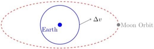
Free Return Trajectory

One of the prettiest features of the Artemis II mission is the use of a free-return trajectory. This type of trajectory is designed so that, even if the spacecraft performs no additional propulsion after the initial injection, it will naturally loop around the Moon and return to Earth.

\[\Delta V_{eff} = \int \mathbf{a}_{Moon} dt\]

The path is determined entirely by the gravitational interaction between the spacecraft, the Earth, and the Moon. As the spacecraft passes near the Moon, its velocity vector is altered by the Moon’s gravitational field. This change is ultimately the cumulative effect of continuous acceleration over time.

Propulsion and Constraints

The ability to execute such a trajectory depends critically on propulsion constraints. The total change in velocity that a rocket can achieve is governed by the Tsiolkovsky rocket equation:

\[\Delta v = v_e \ln \frac{m_0}{m_f}\]

Total energy conservation also plays a vital role in planning the translunar injection:

\[E = \frac{1}{2} m v^2 - \frac{GMm}{r}\]

The precise optimization of these paths often utilizes the Euler-Lagrange framework to minimize fuel consumption:

\[\frac{d}{dt} \left( \frac{\partial L}{\partial \dot{\mathbf{r}}} \right) - \frac{\partial L}{\partial \mathbf{r}} = 0\]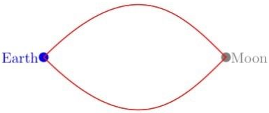

From Apollo to Artemis

Although the mathematical framework underlying Artemis II is the same as that used during the Apollo missions, the implementation has changed significantly. During Apollo, onboard computers had extremely limited processing power, and much of the trajectory planning relied on precomputed solutions and human oversight.

Today, modern missions benefit from advanced numerical methods, high-precision simulations, and real-time trajectory adjustments. The equations have not changed, but the accuracy with which they can be solved and applied has improved dramatically.

Artemis II can essentially be understood as one brutal, high-stakes problem set in celestial mechanics.